Note

This tutorial was generated from a Jupyter notebook that can be downloaded here.

Where’s the spot?

An example of how to solve for the location, amplitude, and size of a star spot.

As we discuss in this notebook, starry isn’t really meant for modeling discrete features such as star spots; rather, starry employs spherical harmonics to model the surface brightness distribution as a smooth, continuous function. We generally recommend approaching the mapping problem in this fashion; see the Eclipsing Binary tutorials for more information on how to do this. However, if you really want to model the surface of a star with star spots, read on!

Let’s begin by importing stuff as usual:

import numpy as np
import starry
import exoplanet as xo
import pymc3 as pm
import pymc3_ext as pmx
import matplotlib.pyplot as plt
from corner import corner

starry.config.quiet = True

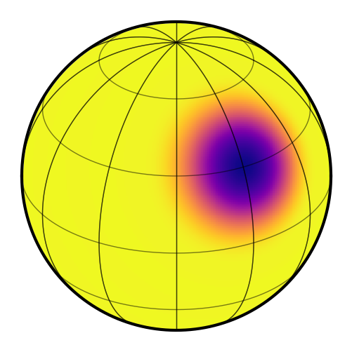
We discussed how to add star spots to a starry map in this tutorial. Here, we’ll generate a synthetic light curve from a star with a single large spot with the following parameters:

# True values
truth = dict(contrast=0.25, radius=20, lat=30, lon=30)

Those are, respectively, the fractional amplitude of the spot, its standard deviation (recall that the spot is modeled as a Gaussian in \(\cos\Delta\theta\), its latitude and its longitude.

To make things simple, we’ll assume we know the inclination and period of the star exactly:

# Things we'll assume are known
inc = 60.0
P = 1.0

Let’s instantiate a 15th degree map and give it those properties:

map = starry.Map(15)
map.inc = inc
map.spot(
    contrast=truth["contrast"],
    radius=truth["radius"],
    lat=truth["lat"],
    lon=truth["lon"],
)
map.show()

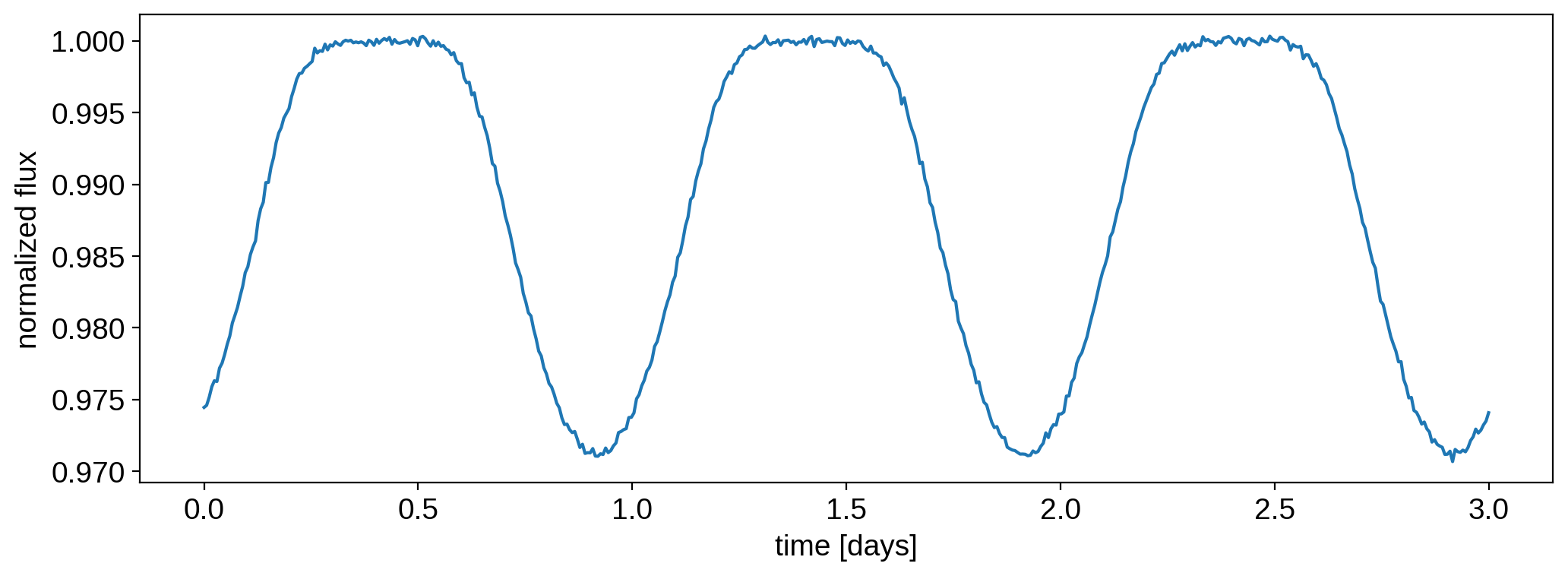
Now we’ll generate a synthetic light curve with some noise:

t = np.linspace(0, 3.0, 500)
flux0 = map.flux(theta=360.0 / P * t).eval()
np.random.seed(0)
flux_err = 2e-4
flux = flux0 + flux_err * np.random.randn(len(t))

Here’s what that looks like:

plt.plot(t, flux)
plt.xlabel("time [days]")
plt.ylabel("normalized flux");

In this notebook, we are going to derive posterior constraints on the spot properties. Let’s define a pymc3 model and within it, our priors and flux model:

with pm.Model() as model:

    # Priors
    contrast = pm.Uniform("contrast", lower=0.0, upper=1.0, testval=0.5)
    radius = pm.Uniform("radius", lower=10.0, upper=35.0, testval=15.0)
    lat = pm.Uniform("lat", lower=-90.0, upper=90.0, testval=0.1)
    lon = pm.Uniform("lon", lower=-180.0, upper=180.0, testval=0.1)

    # Instantiate the map and add the spot
    map = starry.Map(ydeg=15)
    map.inc = inc
    map.spot(contrast=contrast, radius=radius, lat=lat, lon=lon)

    # Compute the flux model
    flux_model = map.flux(theta=360.0 / P * t)
    pm.Deterministic("flux_model", flux_model)

    # Save our initial guess
    flux_model_guess = pmx.eval_in_model(flux_model)

    # The likelihood function assuming known Gaussian uncertainty
    pm.Normal("obs", mu=flux_model, sd=flux_err, observed=flux)

Note

It’s important to define a nonzero testval for both the latitude and longitude of the spot. If you don’t do that, it’s likely the optimizer will get stuck at lat, lon = 0, 0, which is a local maximum of the likelihood.

We’ve placed some generous uniform priors on the four quantities we’re solving for. Let’s run a quick gradient descent to get a good starting position for the sampler:

with model:
    map_soln = pmx.optimize(start=model.test_point)

optimizing logp for variables: [lon, lat, radius, contrast]

100.00% [64/64 00:00<00:00 logp = 3.545e+03]

message: Optimization terminated successfully.
logp: -278193.2524187515 -> 3545.1103694957396

Here’s the data and our initial guess before and after the optimization:

plt.figure(figsize=(12, 5))
plt.plot(t, flux, "k.", alpha=0.3, ms=2, label="data")
plt.plot(t, flux_model_guess, "C1--", lw=1, alpha=0.5, label="Initial")
plt.plot(
    t, pmx.eval_in_model(flux_model, map_soln, model=model), "C1-", label="MAP", lw=1
)
plt.legend(fontsize=10, numpoints=5)
plt.xlabel("time [days]", fontsize=24)
plt.ylabel("relative flux", fontsize=24);

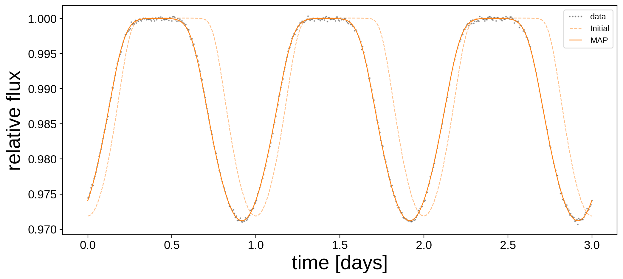
And here are the maximum a posteriori (MAP) values next to the true values:

print("{0:12s} {1:10s} {2:10s}".format("", "truth", "map_soln"))
for key in truth.keys():
    print("{0:10s} {1:10.5f} {2:10.5f}".format(key, truth[key], map_soln[key]))

             truth      map_soln
contrast      0.25000    0.24234
radius       20.00000   20.32443
lat          30.00000   29.83735
lon          30.00000   29.94841

Not bad! Looks like we recovered the correct spot properties. But we’re not done! Let’s get posterior constraints on them by sampling with pymc3. Since this is such a simple problem, the following cell should run in about a minute:

with model:
    trace = pmx.sample(tune=250, draws=500, start=map_soln, chains=4, target_accept=0.9)

Sequential sampling (4 chains in 1 job)
NUTS: [lon, lat, radius, contrast]

100.00% [750/750 00:37<00:00 Sampling chain 0, 0 divergences]

100.00% [750/750 00:38<00:00 Sampling chain 1, 0 divergences]

100.00% [750/750 00:36<00:00 Sampling chain 2, 0 divergences]

100.00% [750/750 00:33<00:00 Sampling chain 3, 0 divergences]

Sampling 4 chains for 250 tune and 500 draw iterations (1_000 + 2_000 draws total) took 146 seconds.

Plot some diagnostics to assess convergence:

var_names = ["contrast", "radius", "lat", "lon"]
display(pm.summary(trace, var_names=var_names))

	mean	sd	hdi_3%	hdi_97%	mcse_mean	mcse_sd	ess_mean	ess_sd	ess_bulk	ess_tail	r_hat
contrast	0.243	0.008	0.228	0.258	0.000	0.000	677.0	677.0	664.0	612.0	1.0
radius	20.326	0.354	19.667	20.987	0.014	0.010	677.0	677.0	666.0	608.0	1.0
lat	29.834	0.158	29.566	30.144	0.005	0.004	1017.0	1017.0	1013.0	1220.0	1.0
lon	29.948	0.044	29.869	30.035	0.001	0.001	1608.0	1608.0	1609.0	1446.0	1.0

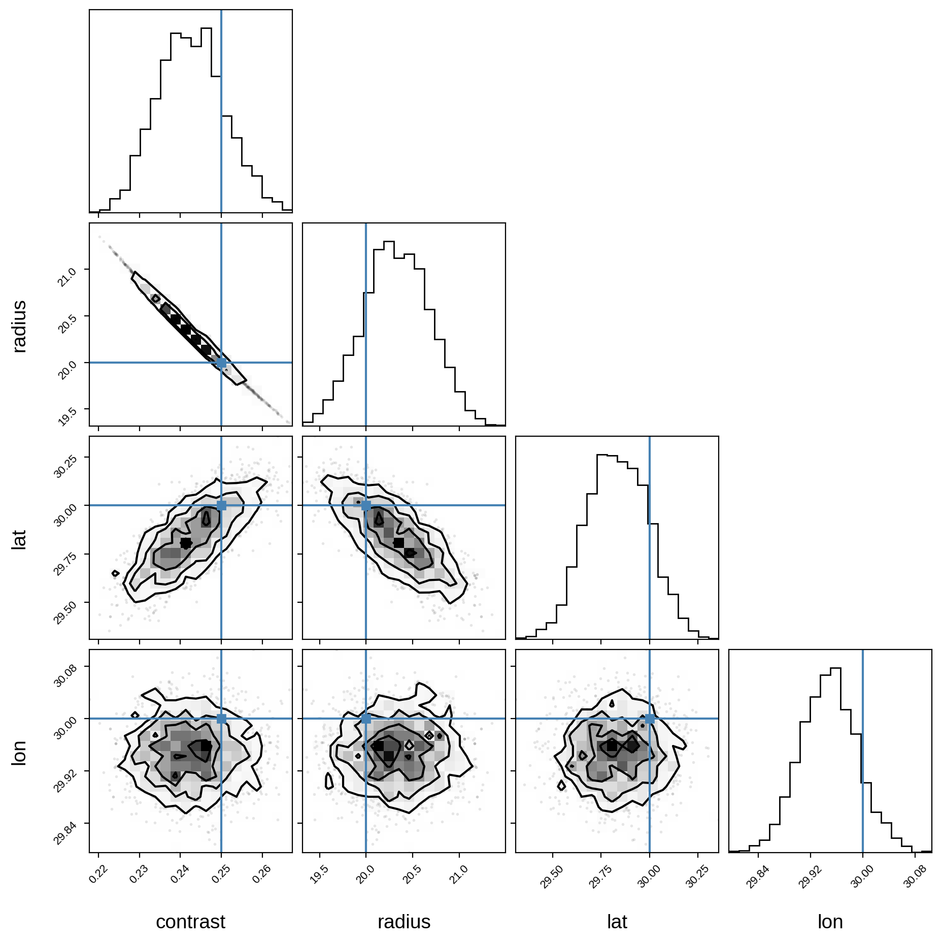
And finally, the corner plot showing the joint posteriors and the true values (in blue):

samples = pm.trace_to_dataframe(trace, varnames=var_names)
corner(samples, truths=[truth[name] for name in var_names]);

WARNING:root:Pandas support in corner is deprecated; use ArviZ directly

We’re done! It’s easy to extend this to multiple spots, simply by calling map.spot once for each spot in the model, making sure you define new pymc3 variables for the spot properties of each spot.