Note
This tutorial was generated from a Jupyter notebook that can be downloaded here.
Marginal likelihood
In the previous notebook we showed how to compute the posterior over maps if we know all other parameters (such as the inclination of the map, the orbital parameters, etc.) exactly. Quite often, however, we do not know these parameters well enough to fix them. In this case, it is often useful to marginalize over all possible maps consistent with the data (and the prior) to compute the marginal likelihood of a given set of parameters. Let’s go over how to do that here.
Generate the data
[3]:
import matplotlib.pyplot as plt
import numpy as np
import starry

np.random.seed(0)
starry.config.lazy = False
starry.config.quiet = True
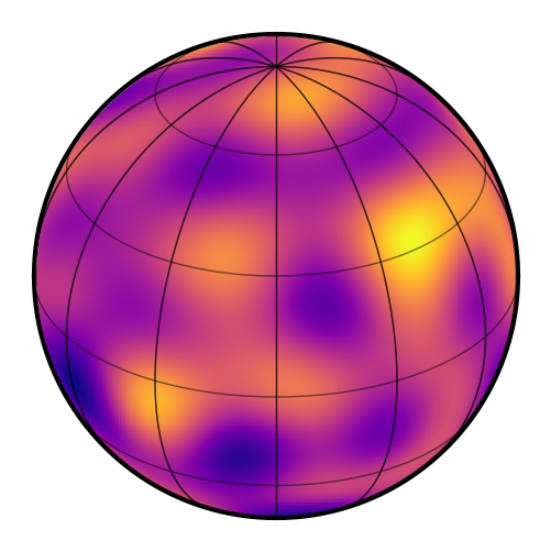
First, we instantiate a map with a random vector of spherical harmonic coefficients. For simplicity, we’ll draw all coefficients from the standard normal. We’ll also give the map an inclination of 60 degrees and a rotation period of one day. In this notebook, we’ll derive a posterior over the inclination and the period by marginalizing over all possible surface maps.
[4]:
map = starry.Map(ydeg=10)
amp_true = 0.9
inc_true = 60.0
period_true = 1.0
map.amp = amp_true
map.inc = inc_true
map[1:, :] = np.random.randn(map.Ny - 1)
map.show()
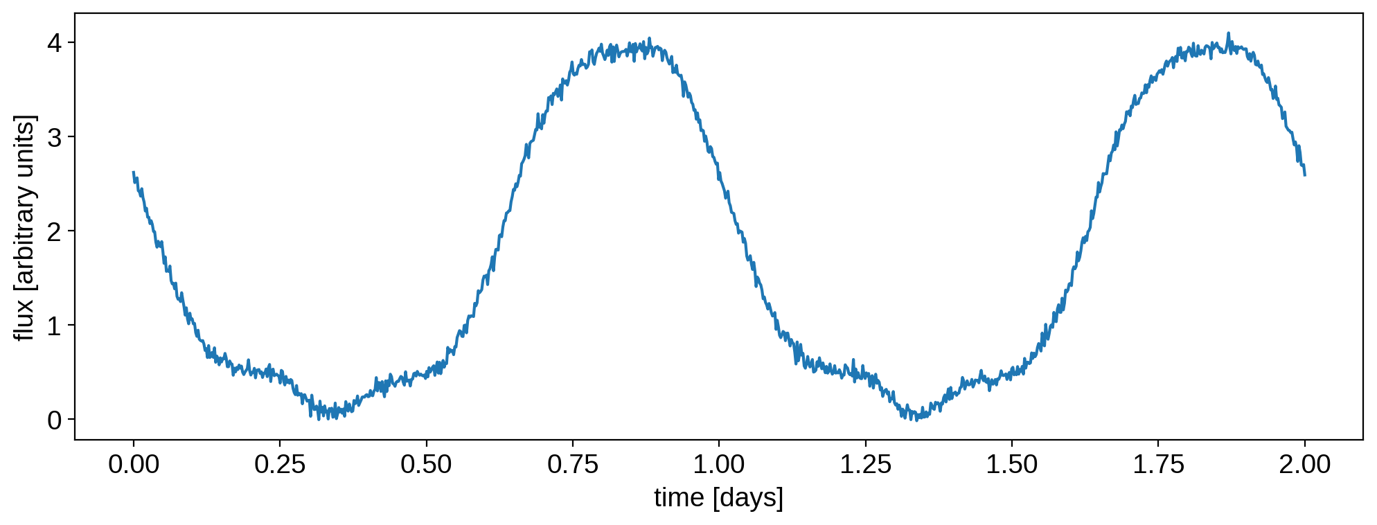
We now generate a synthetic light curve over a couple rotation periods with noise.
[5]:
npts = 1000
sigma = 0.05
time = np.linspace(0, 2, npts)
theta = 360 / period_true * time
flux = map.flux(theta=theta)
flux += np.random.randn(npts) * sigma
[6]:
plt.plot(time, flux)
plt.xlabel(r"time [days]")
plt.ylabel(r"flux [arbitrary units]");
Posterior over inclination
Let’s assume we know the period of the object, and that we know that its spherical harmonic coefficients were all drawn from the unit normal (i.e., we know the power spectrum of the map). But say we don’t know the inclination. What we wish to do is therefore to compute the marginal likelihood of the data for different values of the inclination. Typically the marginal likelihood requires computing a high dimensional integral over all parameters we’re marginalizing over (the 121 spherical
harmonic coefficients in this case), but because the model in starry is linear, this likelihood is analytic!
Let’s specify our data (flux and covariance) and our prior:
[7]:
map.set_data(flux, C=sigma ** 2)
mu = np.zeros(map.Ny)
mu[0] = 1.0
map.set_prior(mu=mu, L=1)
Note that L is the prior covariance matrix, typically denoted \(\Lambda\). In our case it’s just the identity, but if simply we pass a scalar, starry knows to automatically promote it to a diagonal matrix. Same with C, the data covariance: it’s the identity times sigma ** 2.
Next, let’s define a simple function that sets the inclination of the map to a value and returns the corresponding marginal likelihood:
[8]:
def get_lnlike(inc):
    map.inc = inc
    theta = 360 / period_true * time
    return map.lnlike(theta=theta)
Finally, we compute the marginal likelihood over an array of inclinations:
[9]:
%%time
incs = np.linspace(0, 90, 50)
lnlike = np.array([get_lnlike(inc) for inc in incs])
CPU times: user 1.53 s, sys: 212 ms, total: 1.75 s
Wall time: 991 ms
Here’s the likelihood over all possible inclinations. The true value is marked by the vertical line.
[10]:
like = np.exp(lnlike - lnlike.max())
plt.plot(incs, like)
plt.xlabel(r"inclination [deg]")
plt.ylabel(r"relative marginal likelihood")
plt.axvline(inc_true, color="C1", label="true")
plt.legend();
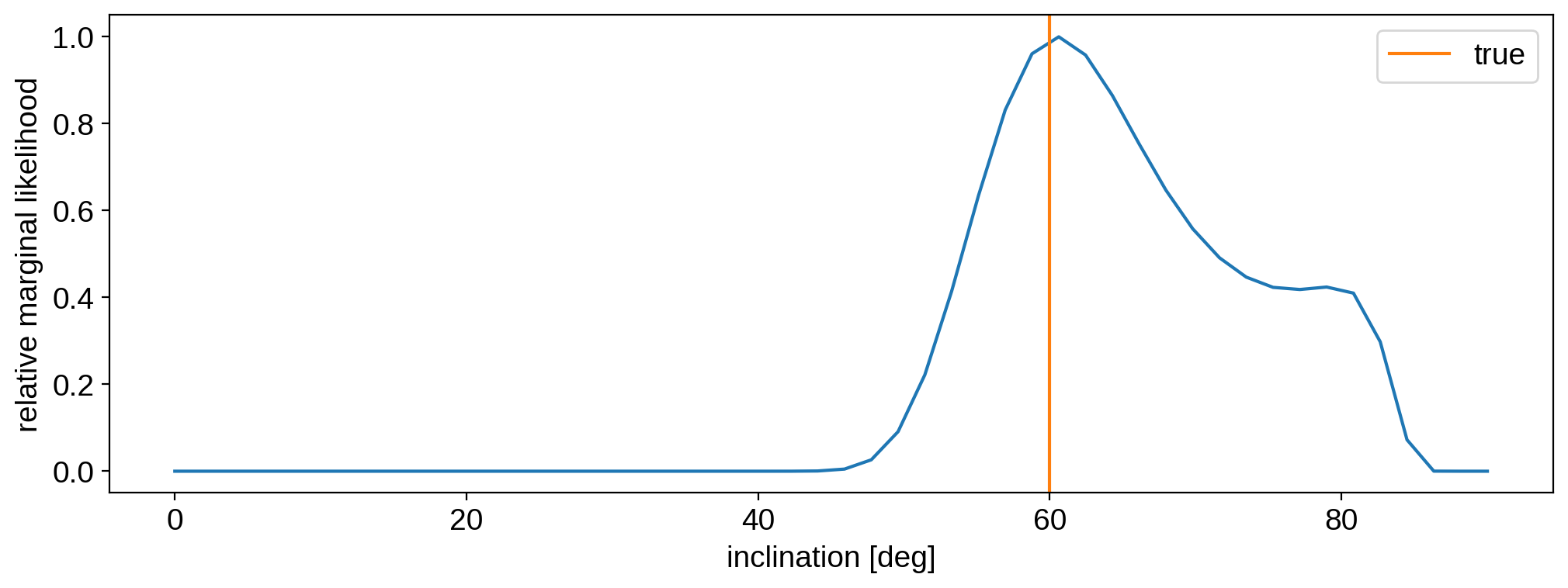
Not bad! Our likelihood function peaks near the true value. To turn this into an actual posterior, we should multiply the likelihood by a prior. A resonable prior to use for inclinations is \(P(i) \propto \sin i\), which is the distribution you’d expect if the rotational angular momentum vector of the object is drawn at random:
[11]:
posterior = like * np.sin(incs * np.pi / 180)
plt.plot(incs, posterior)
plt.xlabel(r"inclination [deg]")
plt.ylabel(r"relative posterior probability")
plt.axvline(inc_true, color="C1", label="true")
plt.legend();
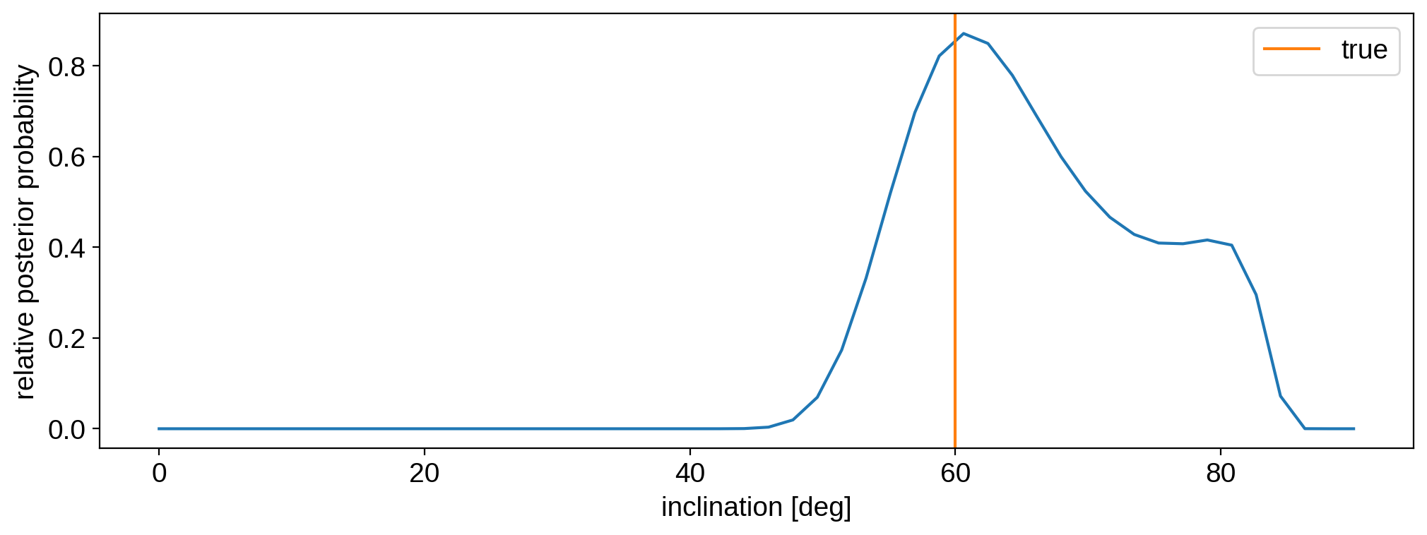
Note that our posterior isn’t correctly normalized (it should integrate to one), but that doesn’t really matter here.
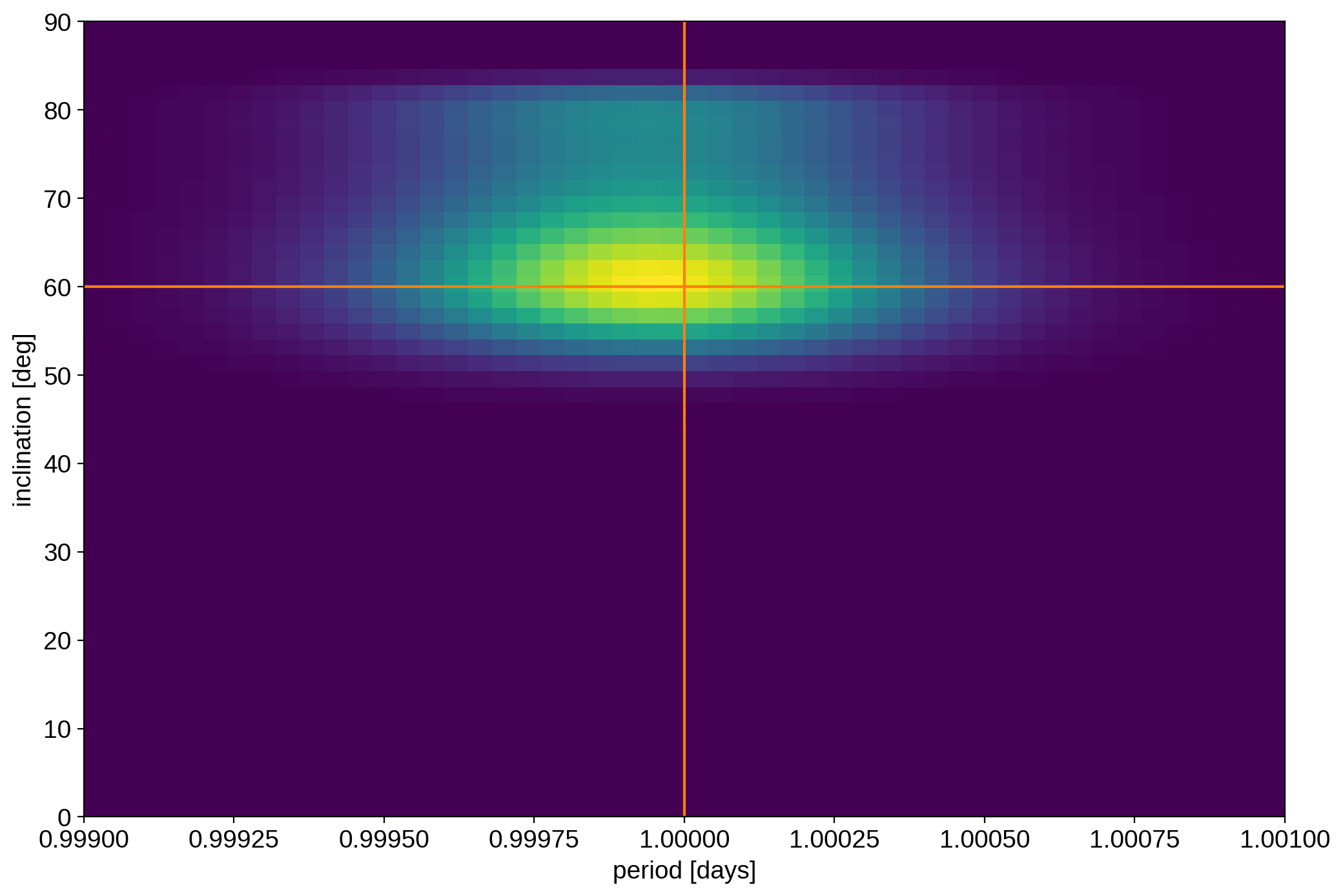
Joint posterior: inclination and period
What if we don’t know either the inclination or the period? We can do the same thing as above, but this time in two dimensions. Let’s redefine our likelihood function to take in the period of the object as well:
[12]:
def get_lnlike(inc, period):
    map.inc = inc
    theta = 360 / period * time
    return map.lnlike(theta=theta)
As we’ll see, the data is very constraining of the period, so let’s do our grid search for period in the range \((0.999, 1.001)\).
[13]:
%%time
incs = np.linspace(0, 90, 50)
periods = np.linspace(0.999, 1.001, 50)

lnlike = np.zeros((50, 50))
for i, inc in enumerate(incs):
    for j, period in enumerate(periods):
        lnlike[i, j] = get_lnlike(inc, period)
CPU times: user 1min 16s, sys: 14.1 s, total: 1min 30s
Wall time: 45.5 s
Let’s again multiply by the inclination sine prior. We’ll assume a flat prior for the period for simplicity.
[14]:
like = np.exp(lnlike - lnlike.max())
posterior = like * np.sin(incs * np.pi / 180).reshape(-1, 1)
Here’s the full joint posterior, marginalized over all possible maps:
[15]:
plt.figure(figsize=(12, 8))
plt.imshow(
    posterior,
    extent=(periods[0], periods[-1], incs[0], incs[-1]),
    origin="lower",
    aspect="auto",
)
plt.axvline(period_true, color="C1")
plt.axhline(inc_true, color="C1")
plt.xlabel("period [days]")
plt.ylabel("inclination [deg]");
That’s it for this tutorial. If you’re thinking of doing this for more than two dimensions, you probably want to turn to sampling with pymc3, as it will probably be more efficient!