Note
This tutorial was generated from a Jupyter notebook that can be downloaded here.
Eclipsing binary: Solving for everything the fast way
In this notebook, we’re continuing our tutorial on how to do inference. In this notebook we showed how to use pymc3 to get posteriors over map coefficients of an eclipsing binary light curve, and in this notebook we did the same thing using the analytic linear formalism of starry. And in the last notebook, we solved for everything at once using pymc3. That was
quite slow: on my 24-core machine, it took 16 hours and 29 minutes to perform 2500 draws in 4 parallel chains. It was also inefficient, and didn’t converge well, as some parameters had a small number of effective samples by the end of the run. That is our target to beat.
In this notebook, we’re going to combine the two methods we discussed previously. We’re going to sample the nonlinear orbital parameters using pymc3 and analytically marginalize over the linear parameters (the spherical harmonic coefficients) using the starry linear formalism.
Note that since we’re using pymc3, we need to enable lazy evaluation mode in starry.
[3]:
import matplotlib
import matplotlib.pyplot as plt
import numpy as np
import pymc3 as pm
import pymc3_ext as pmx
import exoplanet as xo
import os
import starry
from corner import corner
import theano.tensor as tt
from tqdm.notebook import tqdm

np.random.seed(12)
starry.config.lazy = True
starry.config.quiet = True
Load the data
Let’s load the EB dataset:
[5]:
data = np.load("eb.npz", allow_pickle=True)
A = data["A"].item()
B = data["B"].item()
t = data["t"]
flux = data["flux"]
sigma = data["sigma"]
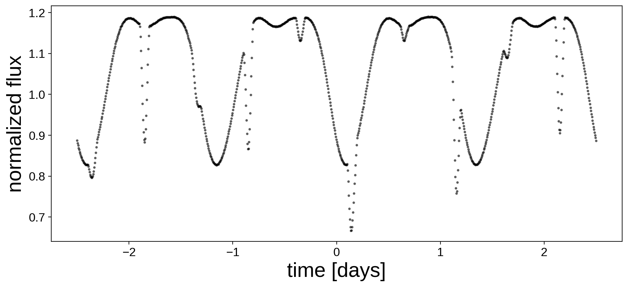
Here’s the light curve we’re going to do inference on:
[6]:
fig, ax = plt.subplots(1, figsize=(12, 5))
ax.plot(t, flux, "k.", alpha=0.5, ms=4)
ax.set_xlabel("time [days]", fontsize=24)
ax.set_ylabel("normalized flux", fontsize=24);
We now instantiate the primary, secondary, and system objects within a pm.Model() context. Here are the priors we are going to assume for the parameters of the primary (same as in the previous notebook):
Parameter |
True Value |
Assumed Value / Prior |
Units |
|---|---|---|---|
\(\mathrm{amp}\) |
\(1.0\) |
\(\mathcal{N}(1.0,0.1^2)\) |
\(-\) |
\(r\) |
\(1.0\) |
\(\mathcal{N}(0.95,0.1^2)\) |
\(R_\odot\) |
\(m\) |
\(1.0\) |
\(\mathcal{N}(1.05,0.1^2)\) |
\(M_\odot\) |
\(P_\mathrm{rot}\) |
\(1.25\) |
\(\mathcal{N}(1.25,0.01^2)\) |
\(\mathrm{days}\) |
\(i\) |
\(80.0\) |
\(\mathcal{N}(80.0,5.0^2)\) |
\(\mathrm{deg}\) |
\(u_1\) |
\(0.40\) |
\(0.40\) |
\(-\) |
\(u_2\) |
\(0.25\) |
\(0.25\) |
\(-\) |
And here are the priors we are going to assume for the secondary (again, same as in the previous notebook):
Parameter |
True Value |
Assumed Value / Prior |
Units |
|---|---|---|---|
\(\mathrm{amp}\) |
\(0.1\) |
\(\mathcal{N}(0.1,0.01^2)\) |
\(-\) |
\(r\) |
\(0.7\) |
\(\mathcal{N}(0.75,0.1^2)\) |
\(R_\odot\) |
\(m\) |
\(0.7\) |
\(\mathcal{N}(0.70,0.1^2)\) |
\(M_\odot\) |
\(P_\mathrm{rot}\) |
\(0.625\) |
\(\mathcal{N}(0.625,0.01^2)\) |
\(\mathrm{days}\) |
\(P_\mathrm{orb}\) |
\(1.0\) |
\(\mathcal{N}(1.01,0.01^2)\) |
\(\mathrm{days}\) |
\(t_0\) |
\(0.15\) |
\(\mathcal{N}(0.15,0.001^2)\) |
\(\mathrm{days}\) |
\(i\) |
\(80.0\) |
\(\mathcal{N}(80.0,5.0^2)\) |
\(\mathrm{deg}\) |
\(e\) |
\(0.0\) |
\(0.0\) |
\(-\) |
\(\Omega\) |
\(0.0\) |
\(0.0\) |
\(\mathrm{deg}\) |
\(u_1\) |
\(0.20\) |
\(0.20\) |
\(-\) |
\(u_2\) |
\(0.05\) |
\(0.05\) |
\(-\) |
Above, \(\mathcal{N}\) denotes a 1-d normal prior with a given mean and variance. Note that for simplicity we are fixing the limb darkening coefficients at their true value.
[7]:
with pm.Model() as model:

    # Some of the gaussians have significant support at < 0
    # Let's force them to be positive (required for quantites
    # such as radius, mass, etc.)
    # NOTE: When using `pm.Bound`, it is *very important* to
    # explicitly define a `testval` -- otherwise this defaults
    # to unity. Since the `testval` is used to initialize the
    # optimization step, it's very important we start at
    # reasonable values, otherwise things will never converge!
    PositiveNormal = pm.Bound(pm.Normal, lower=0.0)

    # Primary
    A_inc = pm.Normal("A_inc", mu=80, sd=5, testval=80)
    A_amp = 1.0
    A_r = PositiveNormal("A_r", mu=0.95, sd=0.1, testval=0.95)
    A_m = PositiveNormal("A_m", mu=1.05, sd=0.1, testval=1.05)
    A_prot = PositiveNormal("A_prot", mu=1.25, sd=0.01, testval=1.25)
    pri = starry.Primary(
        starry.Map(ydeg=A["ydeg"], udeg=A["udeg"], inc=A_inc),
        r=A_r,
        m=A_m,
        prot=A_prot,
    )
    pri.map[1] = A["u"][0]
    pri.map[2] = A["u"][1]

    # Secondary
    B_inc = pm.Normal("B_inc", mu=80, sd=5, testval=80)
    B_amp = 0.1
    B_r = PositiveNormal("B_r", mu=0.75, sd=0.1, testval=0.75)
    B_m = PositiveNormal("B_m", mu=0.70, sd=0.1, testval=0.70)
    B_prot = PositiveNormal("B_prot", mu=0.625, sd=0.01, testval=0.625)
    B_porb = PositiveNormal("B_porb", mu=1.01, sd=0.01, testval=1.01)
    B_t0 = pm.Normal("B_t0", mu=0.15, sd=0.001, testval=0.15)
    sec = starry.Secondary(
        starry.Map(ydeg=B["ydeg"], udeg=B["udeg"], inc=B_inc),
        r=B_r,
        m=B_m,
        porb=B_porb,
        prot=B_prot,
        t0=B_t0,
        inc=B_inc,
    )
    sec.map[1] = B["u"][0]
    sec.map[2] = B["u"][1]

    # System
    sys = starry.System(pri, sec)
Now let’s define our likelihood function. Normally we would call something like pm.Normal to define our data likelihood, but since we’re analytically marginalizing over the surface maps, we use the lnlike method in the System object instead. We pass this to pymc3 via a Potential, which allows us to define a custom likelihood function. Note that in order for this to work we need to set gaussian priors on the spherical harmonic coefficients; see the previous
notebook for more details.
Note, also, that at no point have we set the map coefficients or the amplitude of either object. These are never used – we’re marginalizing over them analytically!
[8]:
with model:
    sys.set_data(flux, C=sigma ** 2)

    # Prior on primary
    pri_mu = np.zeros(pri.map.Ny)
    pri_mu[0] = 1.0
    pri_L = np.zeros(pri.map.Ny)
    pri_L[0] = 1e-2
    pri_L[1:] = 1e-2
    pri.map.set_prior(mu=pri_mu, L=pri_L)

    # Prior on secondary
    sec_mu = np.zeros(pri.map.Ny)
    sec_mu[0] = 0.1
    sec_L = np.zeros(pri.map.Ny)
    sec_L[0] = 1e-4
    sec_L[1:] = 1e-4
    sec.map.set_prior(mu=sec_mu, L=sec_L)

    pm.Potential("marginal", sys.lnlike(t=t))
Now that we’ve specified the model, it’s a good idea to run a quick gradient descent to find the MAP (maximum a posteriori) solution. This will give us a decent starting point for the inference problem.
[9]:
with model:
    map_soln = pmx.optimize()
optimizing logp for variables: [B_t0, B_porb, B_prot, B_m, B_r, B_inc, A_prot, A_m, A_r, A_inc]
124it [00:04, 30.01it/s, logp=5.813719e+03]
CPU times: user 1min, sys: 4.36 s, total: 1min 4s
Wall time: 32 s
message: Desired error not necessarily achieved due to precision loss.
logp: -359099.5579240971 -> 5813.71851514728
To see how we did, let’s plot the best fit solution. We don’t have values for the coefficients (because we marginalized over them), so what we do to get a light curve is we solve for the coefficients (using sys.solve()), conditioned on the best fit values for the orbital parameters. We then set the map coefficients and compute the light curve model using sys.flux(). Note that we need to wrap some things in pmx.eval_in_model() in order to get numerical values out of the pymc3
model.
[10]:
with model:
    x = pmx.eval_in_model(sys.solve(t=t)[0], point=map_soln)
    pri.map.amp = x[0]
    pri.map[1:, :] = x[1 : pri.map.Ny] / pri.map.amp
    sec.map.amp = x[pri.map.Ny]
    sec.map[1:, :] = x[pri.map.Ny + 1 :] / sec.map.amp
    flux_model = pmx.eval_in_model(sys.flux(t=t), point=map_soln)
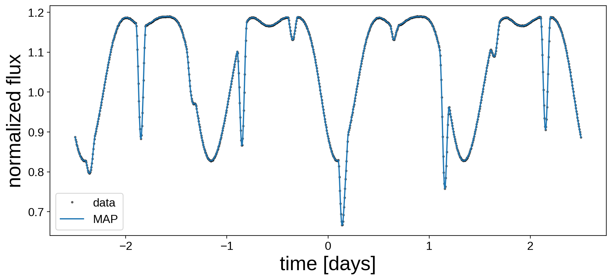
Here’s our model next to the data. We’re doing quite well!
[17]:
fig, ax = plt.subplots(1, figsize=(12, 5))
ax.plot(t, flux, "k.", alpha=0.5, ms=4, label="data")
ax.plot(t, flux_model, "C0", label="MAP")
ax.set_xlabel("time [days]", fontsize=24)
ax.set_ylabel("normalized flux", fontsize=24)
ax.legend();
And here’s what our maps look like. Note that these correspond to the posterior mean of the spherical harmonic coefficients conditioned on the best fitting orbital solution. (Note also that we need to instantiate new maps here so we can visualize them; otherwise pymc3 will complain).
[11]:
map = starry.Map(ydeg=A["ydeg"])
map.inc = map_soln["A_inc"]
map.amp = x[0]
map[1:, :] = x[1 : pri.map.Ny] / map.amp
map.show(theta=np.linspace(0, 360, 50))
[12]:
map = starry.Map(ydeg=B["ydeg"])
map.inc = map_soln["B_inc"]
map.amp = x[pri.map.Ny]
map[1:, :] = x[pri.map.Ny + 1 :] / map.amp
map.show(theta=np.linspace(0, 360, 50))
Not bad! Now the fun part: sampling. Recall that we are analytically marginalizing over the map coefficients and sampling the nonlinear orbital parameters. This will take a while! (But note that sampling usually starts off really slow as the sampler self-tunes, then speeds up quite a bit. The initial time estimate is probably way off!)
[15]:
with model:
    trace = pmx.sample(
        tune=1000, draws=2500, start=map_soln, chains=4, target_accept=0.9
    )
Multiprocess sampling (4 chains in 4 jobs)
NUTS: [B_t0, B_porb, B_prot, B_m, B_r, B_inc, A_prot, A_m, A_r, A_inc]
Sampling 4 chains, 32 divergences: 100%|██████████| 14000/14000 [1:34:18<00:00,  2.47draws/s]
There were 5 divergences after tuning. Increase `target_accept` or reparameterize.
There were 9 divergences after tuning. Increase `target_accept` or reparameterize.
There were 6 divergences after tuning. Increase `target_accept` or reparameterize.
There were 12 divergences after tuning. Increase `target_accept` or reparameterize.
CPU times: user 35.6 s, sys: 3.07 s, total: 38.7 s
Wall time: 1h 34min 26s
This ran much faster than in the previous notebook, where we sampled over the map parameters. We did, however, have divergences and some poor performance along some of the dimensions. But let’s check the diagnostics:
[16]:
var_names_A = ["A_m", "A_r", "A_prot", "A_inc"]
var_names_B = ["B_m", "B_r", "B_porb", "B_prot", "B_inc", "B_t0"]
display(pm.summary(trace, var_names=var_names_A + var_names_B))
| mean | sd | hpd_3% | hpd_97% | mcse_mean | mcse_sd | ess_mean | ess_sd | ess_bulk | ess_tail | r_hat | |
|---|---|---|---|---|---|---|---|---|---|---|---|
| A_m | 1.048 | 0.095 | 0.871 | 1.225 | 0.001 | 0.001 | 4857.0 | 4857.0 | 4840.0 | 5309.0 | 1.0 |
| A_r | 1.026 | 0.029 | 0.974 | 1.083 | 0.000 | 0.000 | 8232.0 | 8232.0 | 8252.0 | 6673.0 | 1.0 |
| A_prot | 1.250 | 0.000 | 1.250 | 1.250 | 0.000 | 0.000 | 10837.0 | 10837.0 | 10851.0 | 7239.0 | 1.0 |
| A_inc | 81.178 | 0.628 | 80.035 | 82.395 | 0.006 | 0.004 | 9905.0 | 9905.0 | 9925.0 | 6969.0 | 1.0 |
| B_m | 0.697 | 0.095 | 0.519 | 0.880 | 0.002 | 0.001 | 2954.0 | 2954.0 | 2940.0 | 2576.0 | 1.0 |
| B_r | 0.692 | 0.023 | 0.650 | 0.735 | 0.000 | 0.000 | 7456.0 | 7456.0 | 7537.0 | 6237.0 | 1.0 |
| B_porb | 1.000 | 0.000 | 1.000 | 1.000 | 0.000 | 0.000 | 6834.0 | 6834.0 | 7012.0 | 6139.0 | 1.0 |
| B_prot | 0.625 | 0.000 | 0.625 | 0.625 | 0.000 | 0.000 | 9490.0 | 9490.0 | 9691.0 | 6449.0 | 1.0 |
| B_inc | 79.843 | 0.277 | 79.327 | 80.371 | 0.003 | 0.002 | 9646.0 | 9646.0 | 9677.0 | 7226.0 | 1.0 |
| B_t0 | 0.150 | 0.000 | 0.150 | 0.150 | 0.000 | 0.000 | 10850.0 | 10850.0 | 10859.0 | 7129.0 | 1.0 |
We actually did pretty well: the r_hat diagnostic is unity and the effective sample size (ess) is several thousand for most parameters. Also much better than in the previous notebook.
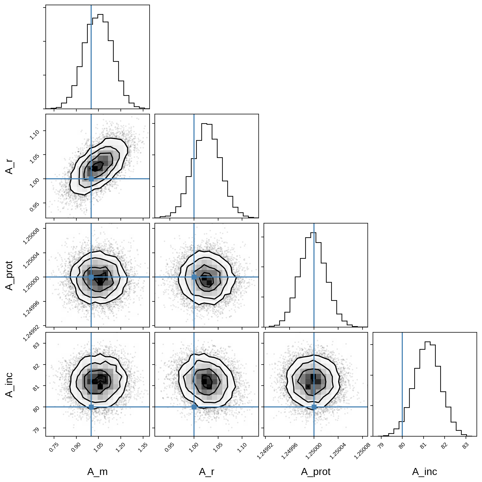
Here’s the corner plot for the posteriors of the primary orbital parameters:
[17]:
truths_A = [A["m"], A["r"], A["prot"], A["inc"]]
samples_A = pm.trace_to_dataframe(trace, varnames=var_names_A)
corner(samples_A, truths=truths_A);
And here’s that same plot for the secondary orbital parameters:
[18]:
truths_B = [B["m"], B["r"], B["porb"], B["prot"], B["inc"], B["t0"]]
samples_B = pm.trace_to_dataframe(trace, varnames=var_names_B)
corner(samples_B, truths=truths_B);
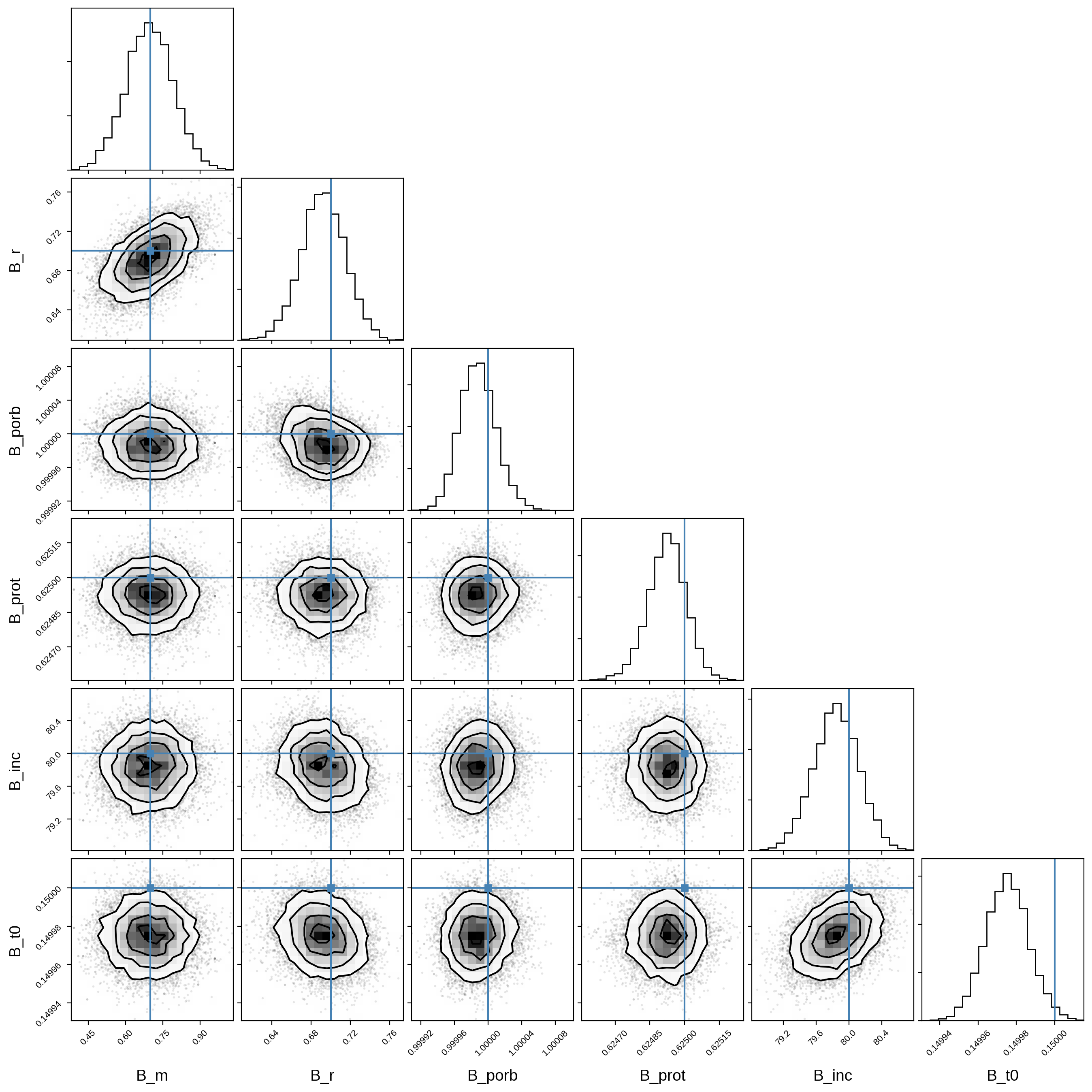
Note that these are qualitatively identical to the ones we derived in the previous notebook (albeit with far more effective samples!)
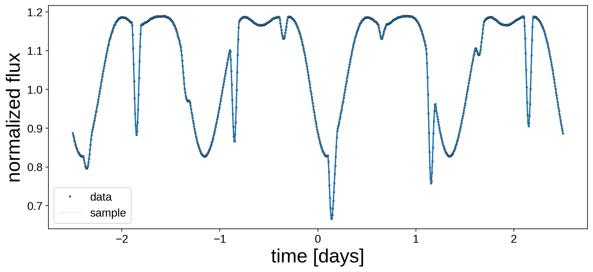
We can verify that our solution is a good fit to the data by drawing random samples and computing the corresponding light curves. We did a similar thing up top, except here we’re actually drawing samples from the map posterior.
Note
The eval_in_model call is really expensive. Stay tuned for a more efficient way of doing this!
[19]:
np.random.seed(1)
nsamples = 30
pri_amp_draw = np.zeros(nsamples)
pri_y_draw = np.zeros((nsamples, pri.map.Ny - 1))
sec_amp_draw = np.zeros(nsamples)
sec_y_draw = np.zeros((nsamples, sec.map.Ny - 1))
flux_model = np.zeros((nsamples, len(t)))
with model:
    for i in tqdm(range(nsamples)):
        idx = np.random.randint(len(trace))
        point = trace.point(idx)
        # Solve the linear problem and draw a sample
        sys.solve(t=t)
        sys.draw()
        # Get the numerical values using `pmx.eval_in_model`
        (
            pri_amp_draw[i],
            pri_y_draw[i],
            sec_amp_draw[i],
            sec_y_draw[i],
            flux_model[i],
        ) = pmx.eval_in_model(
            [pri.map.amp, pri.map[1:, :], sec.map.amp, sec.map[1:, :], sys.flux(t=t)],
            point=point,
        )
[20]:
fig, ax = plt.subplots(1, figsize=(12, 5))
ax.plot(t, flux, "k.", alpha=0.5, ms=4, label="data")
label = "sample"
for i in range(nsamples):
    ax.plot(t, flux_model[i], "C0", label=label, alpha=0.1)
    label = None
ax.set_xlabel("time [days]", fontsize=24)
ax.set_ylabel("normalized flux", fontsize=24)
ax.legend();
Finally, let’s plot the true map next to the mean map and a random sample for each body.
[23]:
map = starry.Map(ydeg=A["ydeg"])
map.amp = np.mean(pri_amp_draw)
map[1:, :] = np.mean(pri_y_draw, axis=0)
pri_mu = map.render(projection="rect").eval()
map.amp = pri_amp_draw[0]
map[1:, :] = pri_y_draw[0]
pri_draw = map.render(projection="rect").eval()
map.amp = A["amp"]
map[1:, :] = A["y"]
pri_true = map.render(projection="rect").eval()

map = starry.Map(ydeg=B["ydeg"])
map.amp = np.mean(sec_amp_draw)
map[1:, :] = np.mean(sec_y_draw, axis=0)
sec_mu = map.render(projection="rect").eval()
map.amp = sec_amp_draw[0]
map[1:, :] = sec_y_draw[0]
sec_draw = map.render(projection="rect").eval()
map.amp = B["amp"]
map[1:, :] = B["y"]
sec_true = map.render(projection="rect").eval()

fig, ax = plt.subplots(3, 2, figsize=(8, 7))
ax[0, 0].imshow(
    pri_true,
    origin="lower",
    extent=(-180, 180, -90, 90),
    cmap="plasma",
    vmin=0,
    vmax=0.4,
)
ax[1, 0].imshow(
    pri_mu,
    origin="lower",
    extent=(-180, 180, -90, 90),
    cmap="plasma",
    vmin=0,
    vmax=0.4,
)
ax[2, 0].imshow(
    pri_draw,
    origin="lower",
    extent=(-180, 180, -90, 90),
    cmap="plasma",
    vmin=0,
    vmax=0.4,
)
ax[0, 1].imshow(
    sec_true,
    origin="lower",
    extent=(-180, 180, -90, 90),
    cmap="plasma",
    vmin=0,
    vmax=0.04,
)
ax[1, 1].imshow(
    sec_mu,
    origin="lower",
    extent=(-180, 180, -90, 90),
    cmap="plasma",
    vmin=0,
    vmax=0.04,
)
ax[2, 1].imshow(
    sec_draw,
    origin="lower",
    extent=(-180, 180, -90, 90),
    cmap="plasma",
    vmin=0,
    vmax=0.04,
)
ax[0, 0].set_title("primary")
ax[0, 1].set_title("secondary")
ax[0, 0].set_ylabel("true", rotation=0, labelpad=20)
ax[1, 0].set_ylabel("mean", rotation=0, labelpad=20)
ax[2, 0].set_ylabel("draw", rotation=0, labelpad=20);
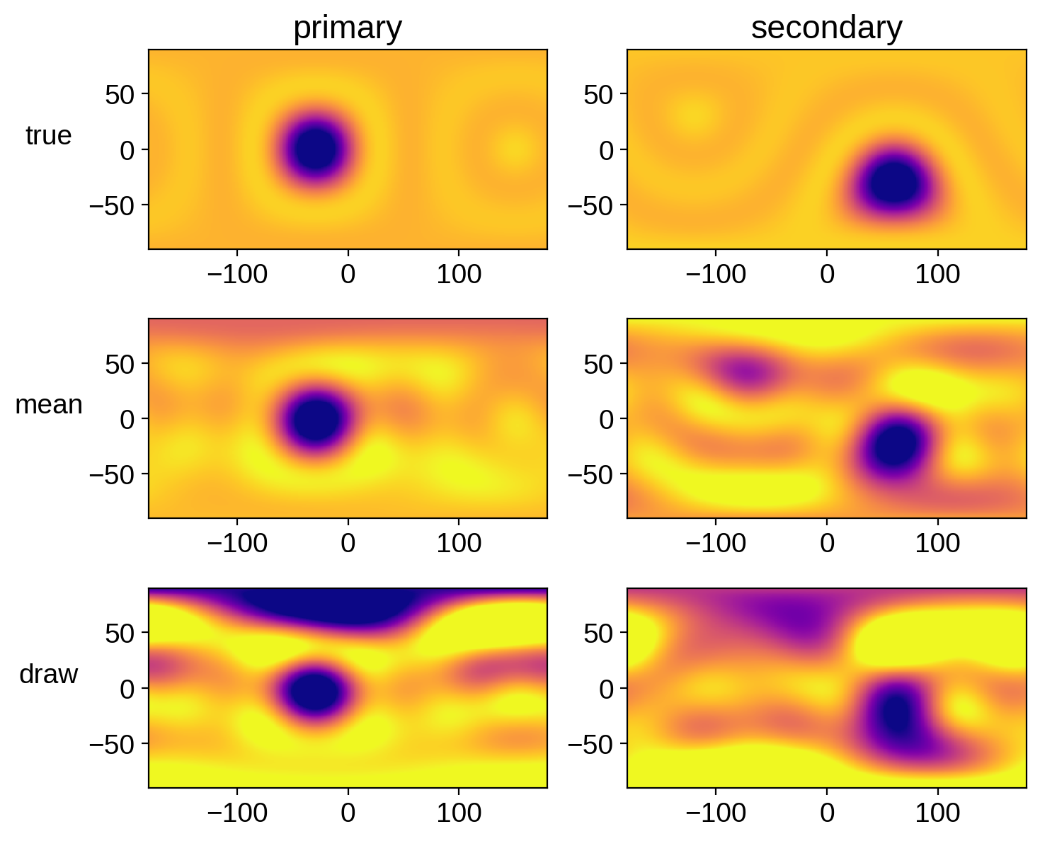
That looks great!