Note

This tutorial was generated from a Jupyter notebook that can be downloaded here.

Doppler imaging: Multi-component maps

In this tutorial, we’ll discuss how to model complex spatial-spectral stellar surfaces by instantiating a multi-component map. This allows us to model a star whose spectrum (not just intensity!) varies with position over the surface in (arbitrarily) complex ways.

Creating a spectral-spatial map

import numpy as np
import matplotlib.pyplot as plt
import starry

We’ll start with a simple example: a star with a single dark spot, whose spectrum is different than the rest of the photosphere. Let’s generate a map of the spot on a 2-dimensional latitude-longitude grid.

lat = np.linspace(-90, 90, 300)
lon = np.linspace(-180, 180, 600)
image = np.ones((len(lat), len(lon)))
y = lat.reshape(-1, 1)
x = lon.reshape(1, -1)
image[x ** 2 + y ** 2 < 30 ** 2] = 0.5

plt.figure(figsize=(10, 4))
plt.imshow(
    image,
    origin="lower",
    cmap="plasma",
    extent=(-180, 180, -90, 90),
    aspect="auto",
)
plt.xticks(np.arange(-180, 180.1, 30))
plt.xlabel("longitude [deg]")
plt.yticks(np.arange(-90, 90.1, 30))
plt.ylabel("longitude [deg]")
plt.grid()
plt.colorbar();

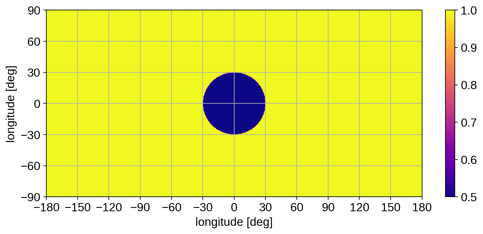
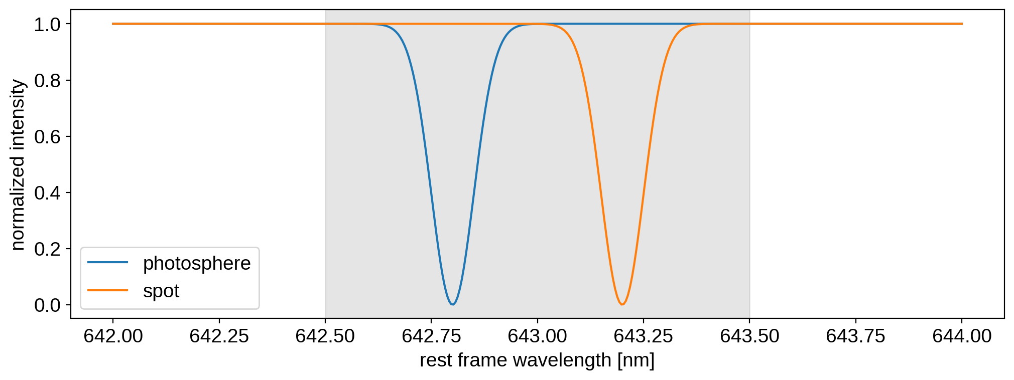
Note that we scaled things so the photosphere has unit intensity and the spot has an intensity of 0.5. Next, let’s define our two spectra: one for the photosphere and one for the spot. For simplicity, we’ll give each spectrum a single Gaussian absorption line, although the location will be different for each component.

wav0 = np.linspace(642.0, 644.0, 400)
wav = np.linspace(642.5, 643.5, 200)
spec1 = 1 - np.exp(-0.5 * (wav0 - 642.8) ** 2 / 0.05 ** 2)
spec2 = 1 - np.exp(-0.5 * (wav0 - 643.2) ** 2 / 0.05 ** 2)

plt.axvspan(wav[0], wav[-1], alpha=0.1, color="k")
plt.plot(wav0, spec1, label="photosphere")
plt.plot(wav0, spec2, label="spot")
plt.xlabel("rest frame wavelength [nm]")
plt.ylabel("normalized intensity")
plt.legend();

Note

Recall the distinction between the rest frame wavelength grid wav0 and the observed wavelength grid wav. The former is the one on which the local, rest frame spectra are defined. The latter is the grid on which we observe the spectrum (after Doppler shifting and integrating over the stellar disk). We don’t actually need wav right now (we’ll use it below). The shaded region indicates the extent of wav; recall that wav0 should typically be padded to avoid edge effects in the convolution step that computes the observed spectra.

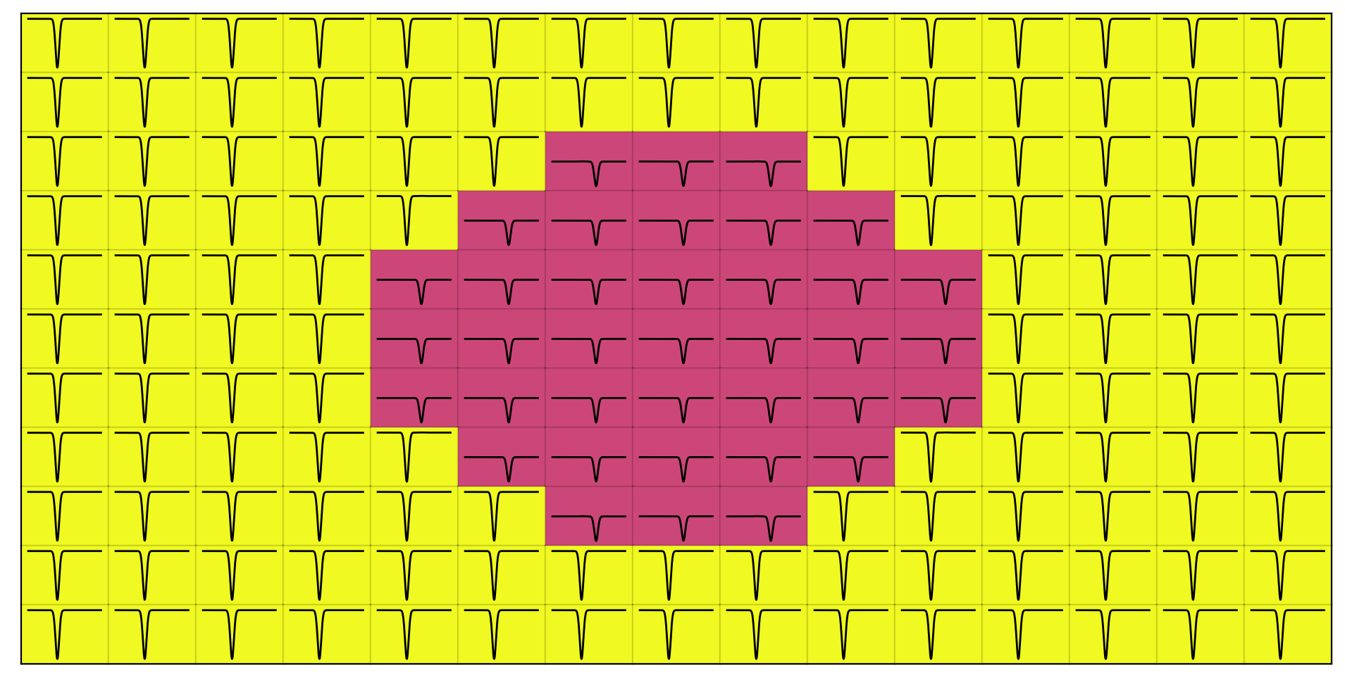
We’re now ready to define the full spectral-spatial stellar surface. Let’s create a data cube: a latitude-longitude grid with a third dimension that contains the spectrum at each point on the surface. We’ll assign each pixel with unit intensity the photospheric spectrum (spec1) and the remaining pixels the spot spectrum (spec2):

cube = np.zeros((len(lat), len(lon), len(wav0)))
bkg = image == 1
cube[bkg, :] = image[bkg].reshape(-1, 1) * spec1.reshape(1, -1)
cube[~bkg, :] = image[~bkg].reshape(-1, 1) * spec2.reshape(1, -1)

Here’s what the (zoomed-in, low-res) cube looks like:

Instantiating the starry model

Now we’re going to load this data cube into a DopplerMap. Let’s instantiate our map as usual, specifying our rest frame and observed wavelength grids, wav and wav0. This time we’ll provide a number of components for the map, nc. In this case, we only need two: one for the photosphere and one for the spot.

map = starry.DopplerMap(15, nc=2, wav=wav, wav0=wav0)

For a little extra flavor, let’s give the star a bit of inclination and a significant equatorial velocity of 30 km/s.

map.inc = 60
map.veq = 30000

Loading our data cube is extremely simple:

map.load(cube=cube)

Internally, starry computes the singular value decomposition (SVD) of the cube to figure out the eigenmaps and eigenspectra defining the stellar surface. Let’s take a look at what we have now:

map.visualize()

Warning

Notebook still under construction. Stay tuned for more!