Note

This tutorial was generated from a Jupyter notebook that can be downloaded here.

The Rossiter-McLaughlin effect

In this notebook, we’ll show how to use starry to model the Rossiter-McLaughlin effect (and radial velocity measurements in general). Check out the notebook on the Derivation of the radial velocity field to understand how starry models radial velocity under the hood.

import matplotlib.pyplot as plt
import starry
import numpy as np
import astropy.units as u

starry.config.lazy = False
starry.config.quiet = True

The basics

To define a radial velocity map, simply pass the rv=True keyword when instantiating a starry Map object. We’ll add quadratic limb darkening just for fun. Note that the spherical harmonic degree ydeg is implicitly set to zero, since we’re not modeling any brightness structure on the surface of the star other than limb darkening (though we can; see below).

map = starry.Map(udeg=2, rv=True)

Next, let’s set the properties that affect the projected radial velocity field. We’ll set the inclination (in degrees), obliquity (also in degrees), equatorial velocity (in meters per second), and the differential rotation shear (unitless):

map.inc = 60
map.obl = 30
map.veq = 1.0e4
map.alpha = 0.3

Let’s also set the limb darkening coefficients:

map[1] = 0.5
map[2] = 0.25

We can see what the map currently looks like. We can choose to either view the brightness map (using rv=False) or the velocity-weighted brightness map (using rv=True). The former is uninteresting, so let’s view the latter:

map.show(rv=True)

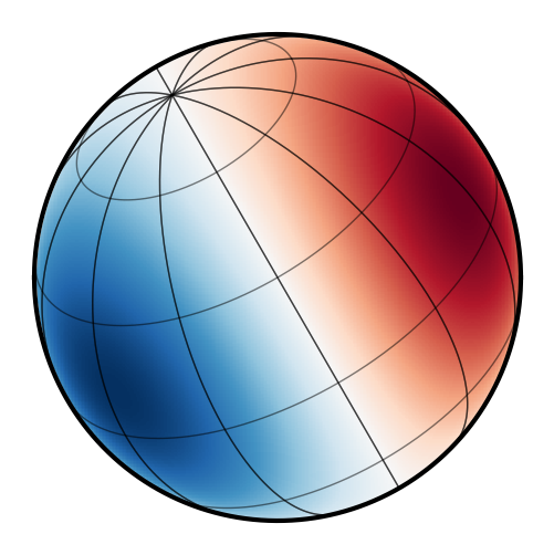
As expected, the map is inclined toward the observer and rotated on the plane of the sky. The left hemisphere is blueshifted (negative radial velocities) and the right hemisphere is redshifted (positive radial velocities). Limb darkening and differential rotation add some additional structure, causing deviations from a perfect dipolar field.

As an example, we can plot what happens when the star is transited by a planet. As usual, we can call map.flux() to get a light curve, but for RV maps we can also call map.rv() to get the radial velocity anomaly one would measure from the object:

# Occultor properties
xo = np.linspace(-1.5, 1.5, 1000)
yo = -0.25
ro = 0.1

# Plot the flux
plt.figure(figsize=(12, 5))
plt.plot(xo, map.flux(xo=xo, yo=yo, ro=ro))
plt.xlabel("Occultor x position [stellar radii]", fontsize=24)
plt.ylabel("Flux [normalized]", fontsize=24)

# Plot the radial velocity
plt.figure(figsize=(12, 5))
plt.plot(xo, map.rv(xo=xo, yo=yo, ro=ro))
plt.xlabel("Occultor x position [stellar radii]", fontsize=24)
plt.ylabel("Radial velocity [m/s]", fontsize=24);

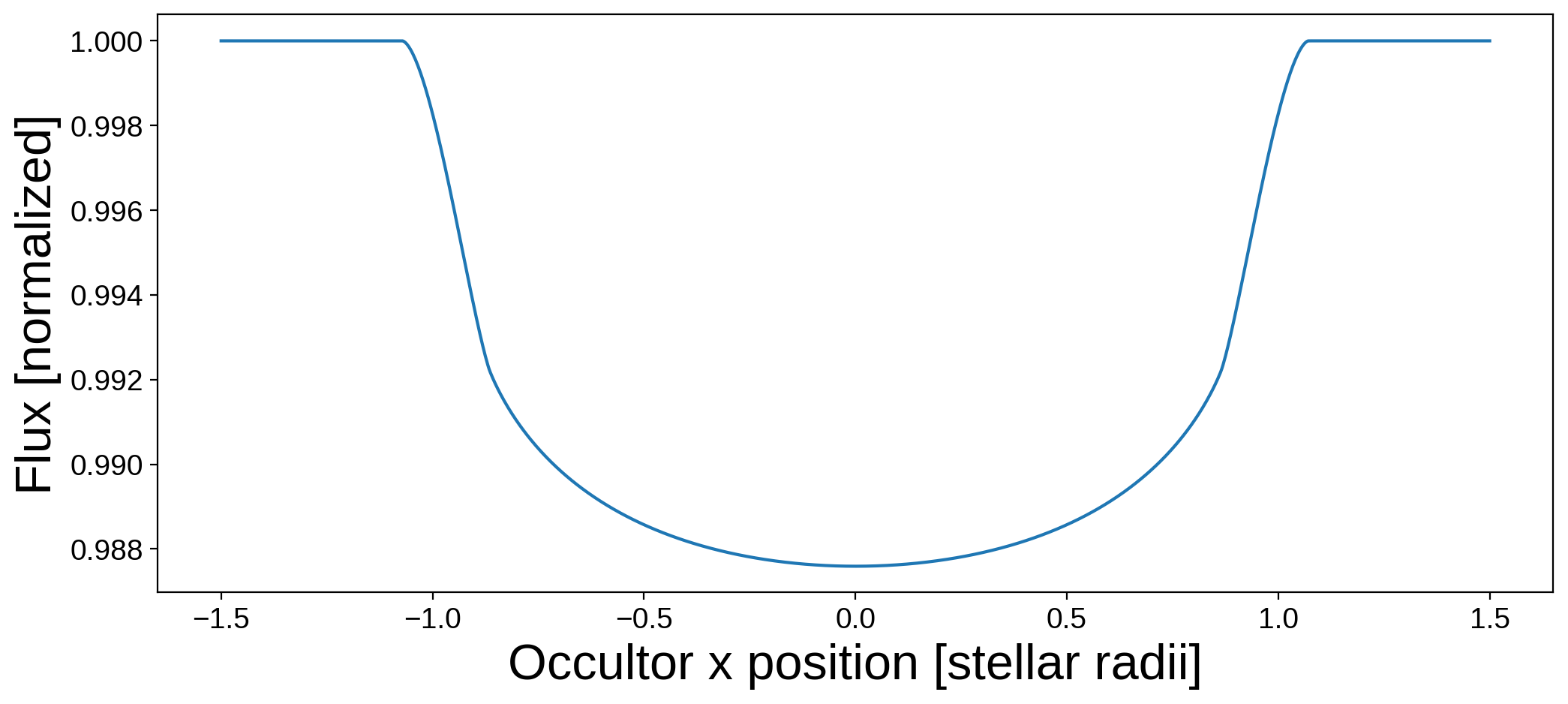
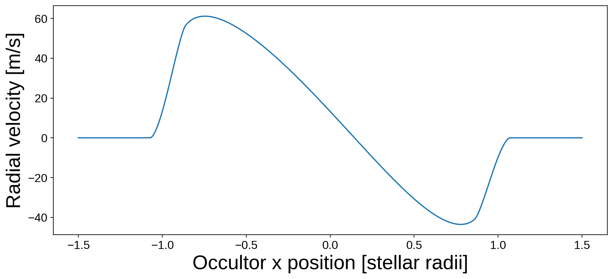
The first plot is the usual transit light curve, and the second plot is the Rossiter-McLaughlin effect. Note that the units of the RV in the second plot are given by map.velocity_units.

Accounting for surface features

The effect of a planet occulting a star on the observed radial velocity is similar to that of a spot rotating in and out of view. With starry, we can model both using the same formalism. Let’s define a map of a higher spherical harmonic degree to model the effect of a spot on the RV measurements:

map = starry.Map(ydeg=10, udeg=2, rv=True)

We’ll give it the same properties as before:

map.inc = 60
map.obl = 30
map.veq = 1.0e4
map.alpha = 0.3
map[1] = 0.5
map[2] = 0.25

And this time we’ll also add a large spot:

map.add_spot(-0.015, sigma=0.03, lat=30, lon=0)

Here’s what the map looks like in white light:

map.show(rv=False, theta=np.linspace(0, 360, 50))

And here’s what it looks like in velocity space:

map.show(rv=True, theta=np.linspace(0, 360, 50))

Let’s plot the light curve and the radial velocity anomaly for this map over one rotation period:

theta = np.linspace(-180, 180, 1000)

# Plot the flux
plt.figure(figsize=(12, 5))
plt.plot(theta, map.flux(theta=theta))
plt.xlabel("Angle of rotation [degrees]", fontsize=24)
plt.ylabel("Flux [normalized]", fontsize=24)

# Plot the radial velocity
plt.figure(figsize=(12, 5))
plt.plot(theta, map.rv(theta=theta))
plt.xlabel("Angle of rotation [degrees]", fontsize=24)
plt.ylabel("Radial velocity [m/s]", fontsize=24);

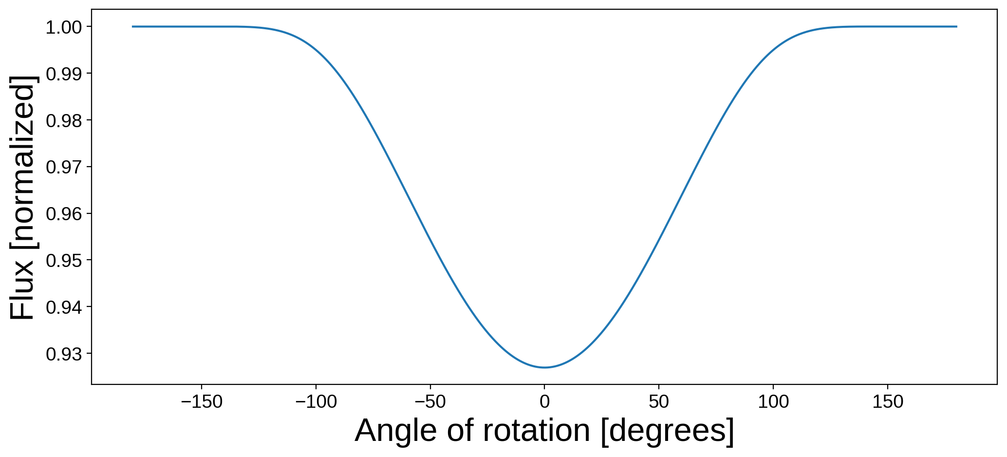
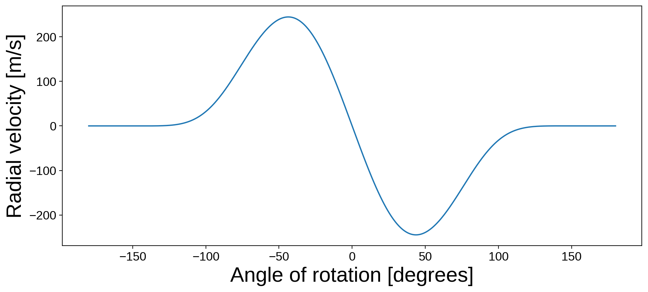
As expected, the signal is similar to the Rossiter-McLaughlin effect! Note that this is a very simple version of Doppler imaging, as we are modeling only the observed radial velocity — not any details of the line shape changes due to the spot rotating in and out of view. This feature of starry is therefore not meant to enable the mapping of stellar surfaces from RV data, but it can be used to model the RV effects of spots on the surface for, say, de-trending radial velocity observations when modeling planetary signals.

The full RV model

So far we’ve shown how to manually specify the occultor properties and position to get the Rossiter-McLaughlin signal, but we can use the formalism of starry.System to model a full system of Keplerian bodies.

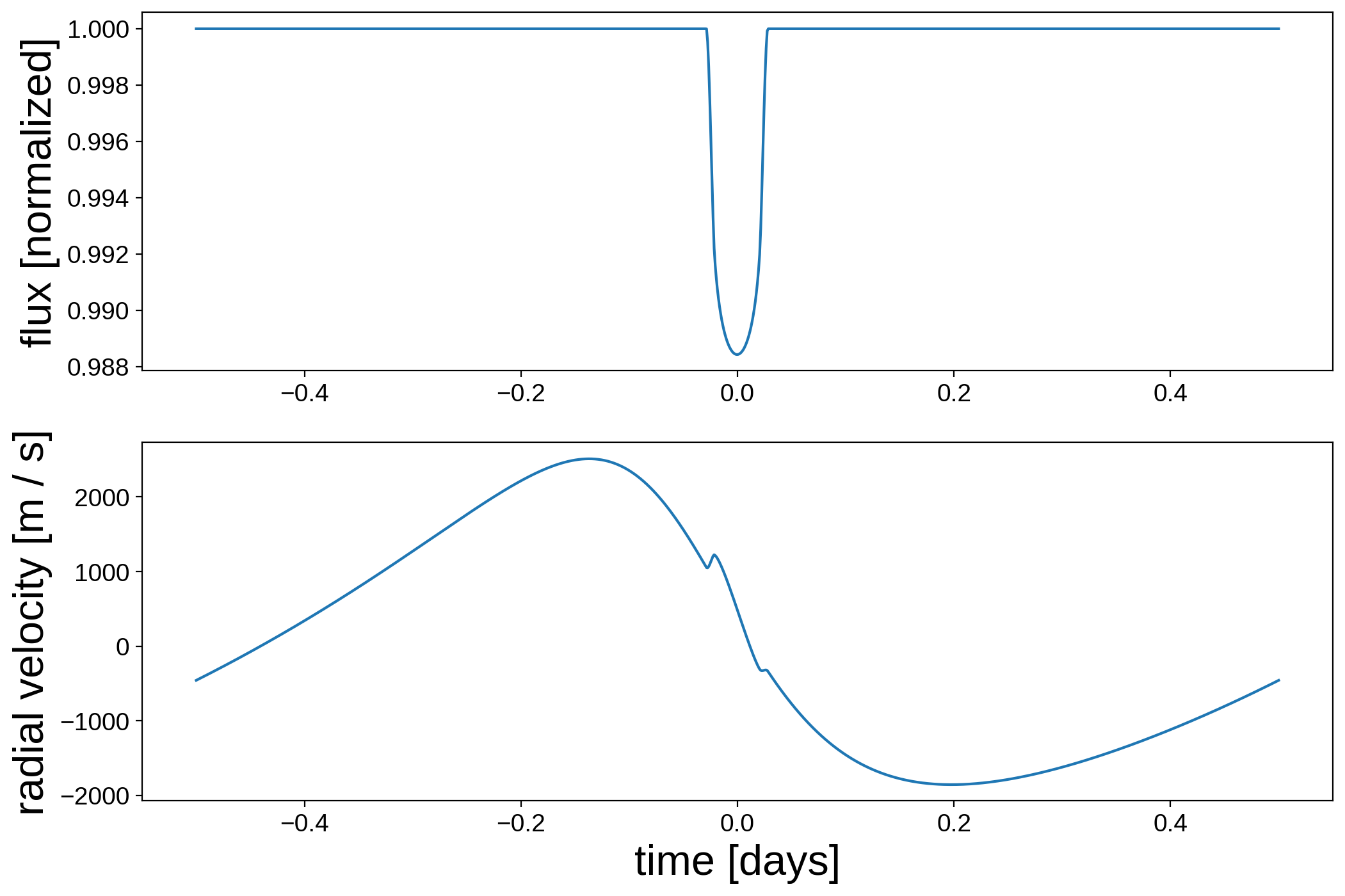
Here’s an example of a misaligned hot Jupiter on an eccentric orbit, where we compute both the flux and the radial velocity:

# Define the star
A = starry.Primary(
    starry.Map(udeg=2, rv=True, amp=1, veq=5e4, alpha=0, obl=30),
    r=1.0,
    m=1.0,
    length_unit=u.Rsun,
    mass_unit=u.Msun,
)
A.map[1] = 0.5
A.map[2] = 0.25

# Define the planet
b = starry.Secondary(
    starry.Map(rv=True, amp=0, veq=0),
    r=0.1,
    porb=1.0,
    m=0.01,
    t0=0.0,
    inc=80.0,
    ecc=0.3,
    w=60,
    length_unit=u.Rsun,
    mass_unit=u.Msun,
    angle_unit=u.degree,
    time_unit=u.day,
)

# Define the system
sys = starry.System(A, b)

# Compute the flux & RV signal
time = np.linspace(-0.5, 0.5, 1000)
flux = sys.flux(time)
rv = sys.rv(time)

# Plot it
fig, ax = plt.subplots(2, figsize=(12, 8))
ax[0].plot(time, flux)
ax[1].plot(time, rv)
ax[1].set_xlabel("time [days]", fontsize=24)
ax[0].set_ylabel("flux [normalized]", fontsize=24)
ax[1].set_ylabel("radial velocity [m / s]", fontsize=24);