Note

This tutorial was generated from a Jupyter notebook that can be downloaded here.

Map orientation

Below we discuss various things relating to the orientation of the surface maps in starry.

import matplotlib.pyplot as plt
import numpy as np
import starry

starry.config.lazy = False
starry.config.quiet = True

Inclination and obliquity of Map instances

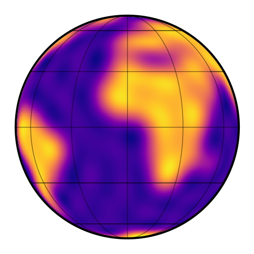
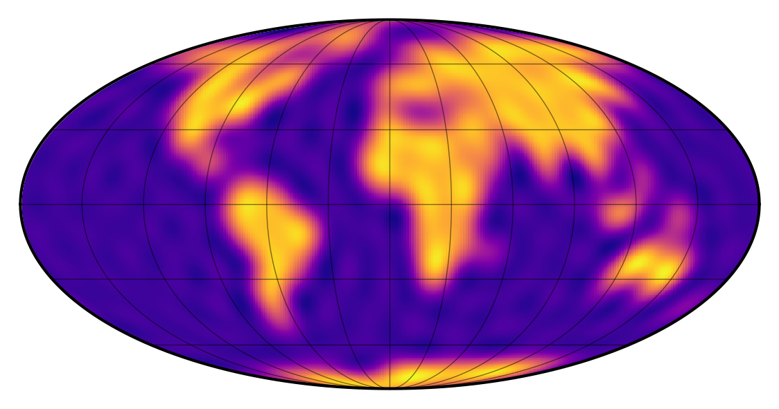
Let’s construct a 20th-degree map and load the continental map of the Earth.

ydeg = 20
earth_map = starry.Map(ydeg=ydeg, quiet=True)
earth_map.load("earth", sigma=0.075)
earth_map.show()

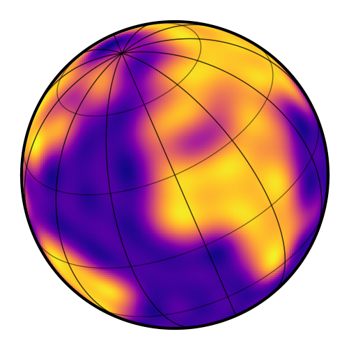
Now, just as an example, let’s give the Earth an obliquity of 23.5 degrees and an inclination of 60 degrees. In the previous version of starry, we did this by setting the axis property, but now we can directly set the inclination inc and obliquity obl.

earth_map.obl = 23.5
earth_map.inc = 60.0
earth_map.show()

Several comments about what we just did:

1. We specified the angles in degrees

That’s because the default angular unit for maps is

earth_map.angle_unit

$\mathrm{{}^{\circ}}$

(i.e., degrees). We could change that to radians by specifying

from astropy import units as u
earth_map.angle_unit = u.radian

2. Definition of the angles

In starry we define the obliquity to be the angle of rotation on the sky, measured counter-clockwise from north. The inclination is the angle between the axis of rotation and the line of sight (the usual definition for exoplanets).

3. The inclination and obliquity specify the vantage point of the observer

In the previous version of starry, changing the axis of rotation of the map changed the actual location of the rotational poles on the surface. In other words, the axis of rotation was an intrinsic property of the map, specifying the location of the poles in the observer’s reference frame. That has changed in version 1.0. The axis of rotation (determined by inc and obl) is now a property of the observer; changing these values change the angle at which the map is seen by the observer. The location of the poles on the surface of the body therefore remain fixed.

This change is due to the fact that as of starry 1.0, the spherical harmonic coefficients are defined relative to the rotational axis of the map in a static, observer-independent frame. Changing the map inclination or obliquity merely changes the vantage point of the observer, not the spherical harmonic coefficients.

4. The show method

Finally, note that the show() method can also animate the map as it rotates:

theta = np.linspace(0, 360, 50)
earth_map.show(theta=theta)

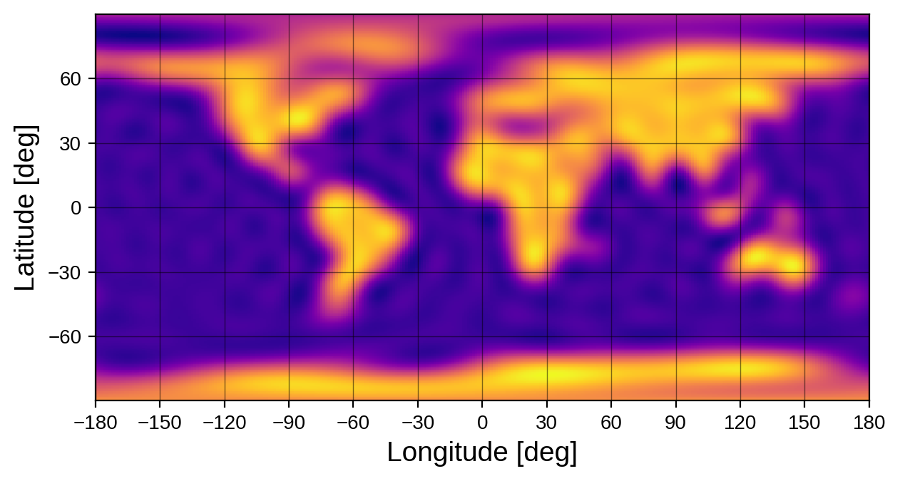
It can also plot an equi-rectangular (latitude-longitude) view of the map:

earth_map.show(projection="rect")

as well as a Mollweide view:

earth_map.show(projection="moll")

Inclination and obliquity of Secondary instances

Understanding the inclination and obliquity of a standalone Map instance is straightforward. But things can get a little tricky when we’re modeling the surface map of a body in a Keplerian orbit, since we have the orbital inclination (\(i\)) and obliquity (\(\Omega\), usually called the longitude of ascending node) to worry about as well.

The thing to remember is this: the inc and obl attributes of the map tell you everything you need to know about the orientation of the surface map on the sky. Changing the inclination and longitude of ascending node of the body only affects the orientation of the orbit, not the orientation of the map.

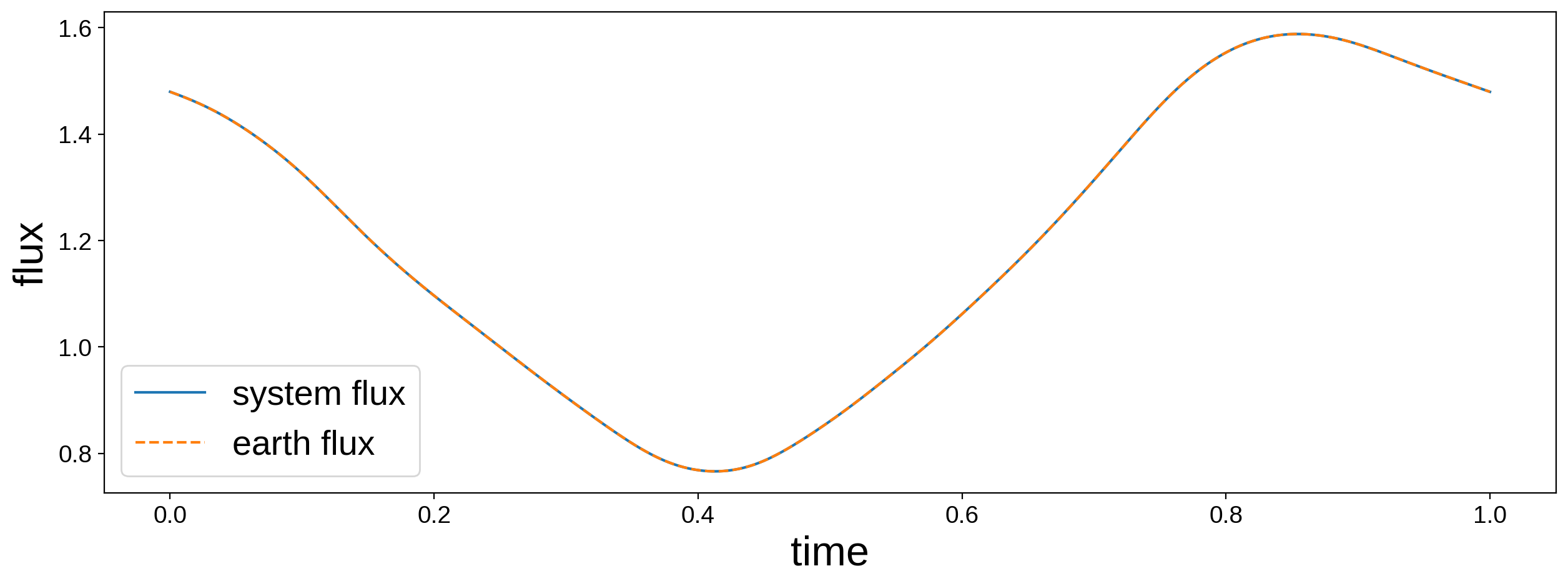
Below, we instantiate a Keplerian system using the Earth map (inclination \(60^\circ\) and obliquity \(23.5^\circ\)) defined above. We give the planet an inclination of \(45^\circ\) and a longitude of ascending node of \(10^\circ\). However, as we will see, when we compute the system flux, we get the same light curve as before: the light curve of the Earth rotating at inclination \(60^\circ\) and obliquity \(23.5^\circ\).

# Define the Earth-Sun system
sun = starry.Primary(starry.Map(amp=0.0))
earth = starry.Secondary(earth_map, porb=1.0, r=0.01, inc=45.0, Omega=10.0)
sys = starry.System(sun, earth)
t = np.linspace(0, 1, 1000)

# Plot the system light curve
fig = plt.figure(figsize=(15, 5))
plt.plot(t, sys.flux(t), label="system flux")

# Plot just the Earth's light curve
plt.plot(t, earth_map.flux(theta=360.0 * t), "--", label="earth flux")

# Labels
plt.xlabel("time", fontsize=24)
plt.ylabel("flux", fontsize=24)
plt.legend(fontsize=20);

To recap, let’s say we define the following Secondary instance:

planet = starry.Secondary(
    starry.Map(
        inc=inc_map,
        obl=obl_map
    ),
    inc=inc_orb,
    Omega=Omega_orb
)

There are four angles to be aware of: two associated with the Map instance (inc_map and obl_map), and two associated with the Secondary instance (inc_orb and Omega_orb). The first two define the orientation of the surface map on the sky, and the last two define the orientation of the orbit on the sky. Unfortunately, both the map and orbital inclinations have the same name, but one is a keyword argument to Map and one is a keyword argument to Secondary. Another, perhaps less confusing, way to define this system is as follows:

planet = starry.Secondary(starry.Map())
planet.map.inc = inc_map
planet.map.obl = obl_map
planet.inc = inc_orb
planet.Omega = Omega_orb

While this convention is nice because it decouples the orbit from the rotation of the planet, it is often the case that the orbital plane and the equatorial plane are the same (such as for a tidally locked planet), in which case the two inclinations and the two obliquities are the same. In this case, we can explicitly set them equal to each other:

planet = starry.Secondary(starry.Map())
planet.inc = planet.map.inc
planet.Omega = planet.map.obl

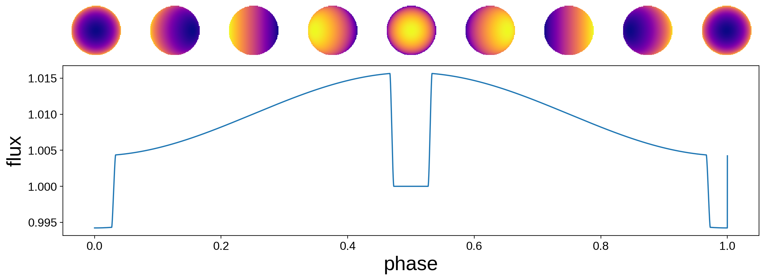
The rotational phase of Secondary instances

Finally, we must also be careful about the rotational phase theta of the map when using Secondary instances. All Secondary instances have a theta0 parameter, which specifies the rotational phase of the map at time t0 (also a property of all Secondary instances). By default, theta0 = 0, so when t = t0 (whose default value is also zero), the line of sight vector intersects the prime meridian (longitude zero) of the map.

The parameter t0 also specifies the time of transit (or inferior conjunction, if the body does not transit), so if theta0 is kept at its default value of zero, the map coefficients describe what the body looks like if it were viewed by an observer seeing the system edge on while the secondary body is transiting. Note that this is different from the convention adopted in the beta (0.3.0) version.

Let’s look at an example. Below we instantiate a simple tidally-locked star-planet system.

star = starry.Primary(starry.Map())
planet = starry.Secondary(starry.Map(ydeg=1, amp=0.01), porb=1.0, prot=1.0, r=0.1)
sys = starry.System(star, planet)
t = np.linspace(0, 1, 10000)

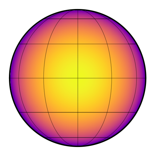
We will give the planet a simple dipole map:

planet.map[1, 0] = 0.5

In the static frame, this corresponds to the following surface map:

planet.map.show()

By default, the inclination of the orbit (and of the map) is \(90^\circ\), and t0, theta0, and the eccentricity are all zero. Here’s what the system light curve looks like, along with the orientation of the map at several points in time:

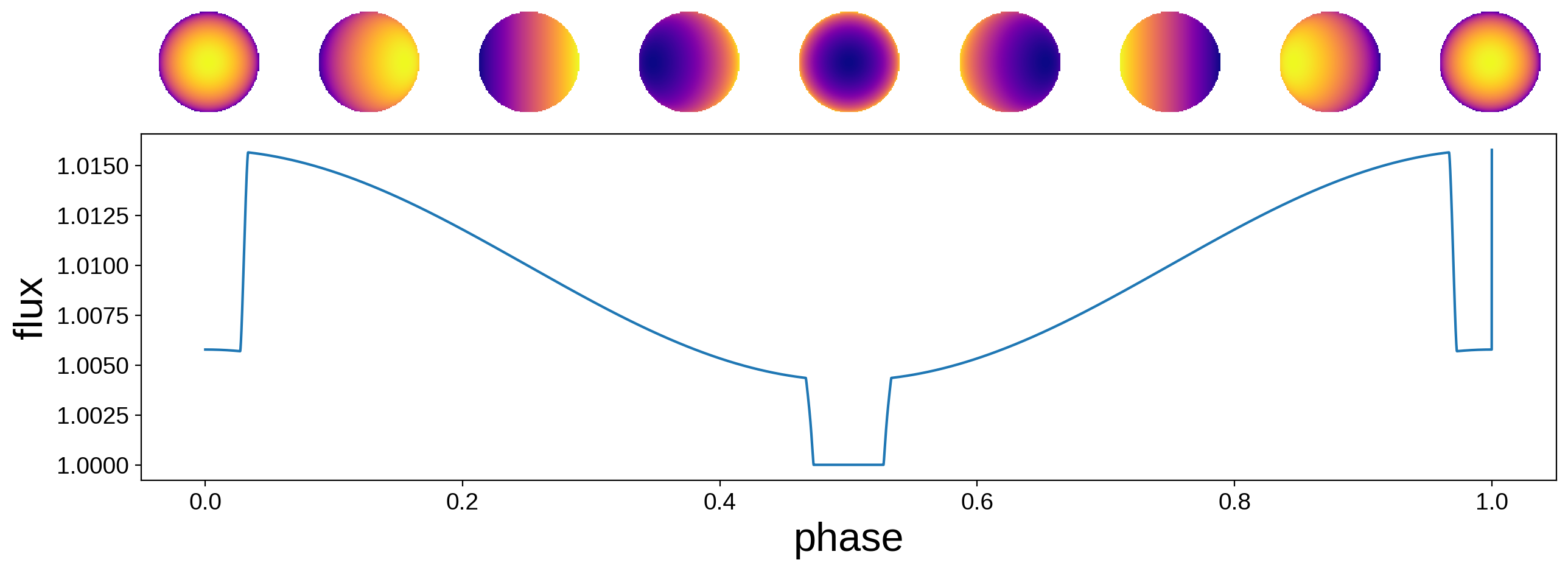
The transit occurs at \(t = 0\) (and \(t = 1\)) and the secondary eclipse occurs at \(t = 0.5\). As we mentioned above, at \(t = t_0\) the map is at its initial phase. Since t0 corresponds to a transiting configuration, the bright side of the planet is facing away from the star and toward the observer at this time. This is probably undesirable, since normally we’d expect the bright side of the planet to face the star.

The easiest way around this is to add a \(180^\circ\) phase offset via the theta0 parameter:

planet.map[1, 0] = 0.5
planet.theta0 = 180