Note

This tutorial was generated from a Jupyter notebook that can be downloaded here.

Staying Positive

Unfortunately, there’s no trivial way of setting the spherical harmonic coefficients to ensure the map intensity is non-negative everywhere. One helpful thing to keep in mind is that the average intensity across the surface does not change when you modify the spherical harmonic coefficients. That’s because all spherical harmonics other than \(Y_{0,0}\) are perfectly anti-symmetric: for every bright region on the surface, there’s an equally dark region on the other side that cancels its contribution to the surface-integrated intensity. What this means is that the magnitude of the spherical harmonic coefficients controls the departure of the intensity from this mean value (which is equal to the intensity of the \(Y_{0,0}\) harmonic, \(\frac{1}{\pi}\)). One way to ensure the map is non-negative everywhere is therefore simply to limit the amplitude of all spherical harmonic coefficients to a small value.

Spherical harmonic maps

However, in some cases it might be useful to check in the general case whether or not a map is positive semi-definite. This entails running a nonlinear minimization on the intensity across the surface. For spherical harmonic maps, this is implemented in the minimize() method. Let’s import starry, instantiate a map, and take a look.

import numpy as np
import matplotlib.pyplot as plt
import starry

starry.config.lazy = False
starry.config.quiet = True

Let’s set the coefficients randomly…

map = starry.Map(ydeg=5)
np.random.seed(0)
map[1:, :] = 0.1 * np.random.randn(map.Ny - 1)

… and plot the map on a lat-lon grid:

image = map.render(projection="rect")
plt.imshow(image, origin="lower", cmap="plasma", extent=(-180, 180, -90, 90))
plt.xlabel("longitude [deg]")
plt.ylabel("latitude [deg]")
plt.colorbar();

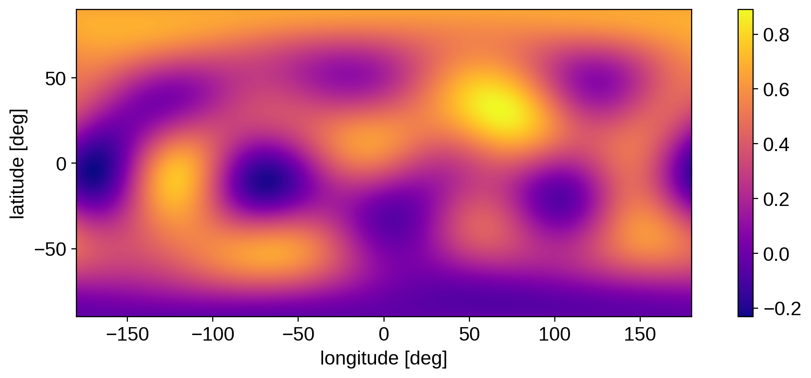
The map clearly goes negative in certain regions. If we call minimize(), we can get the latitude, longitude, and value of the intensity at the minimum:

%%time
lat, lon, value = map.minimize()

CPU times: user 5.63 ms, sys: 0 ns, total: 5.63 ms
Wall time: 4.83 ms

print(lat, lon, value)

-4.314289159079777 -170.46917574859165 -0.23198456828161299

plt.imshow(image, origin="lower", cmap="plasma", extent=(-180, 180, -90, 90))
plt.xlabel("longitude [deg]")
plt.ylabel("latitude [deg]")
plt.axvline(lon, color="k", ls="--")
plt.axhline(lat, color="k", ls="--")
plt.title("minimum: {0:.3f}".format(value))
plt.colorbar();

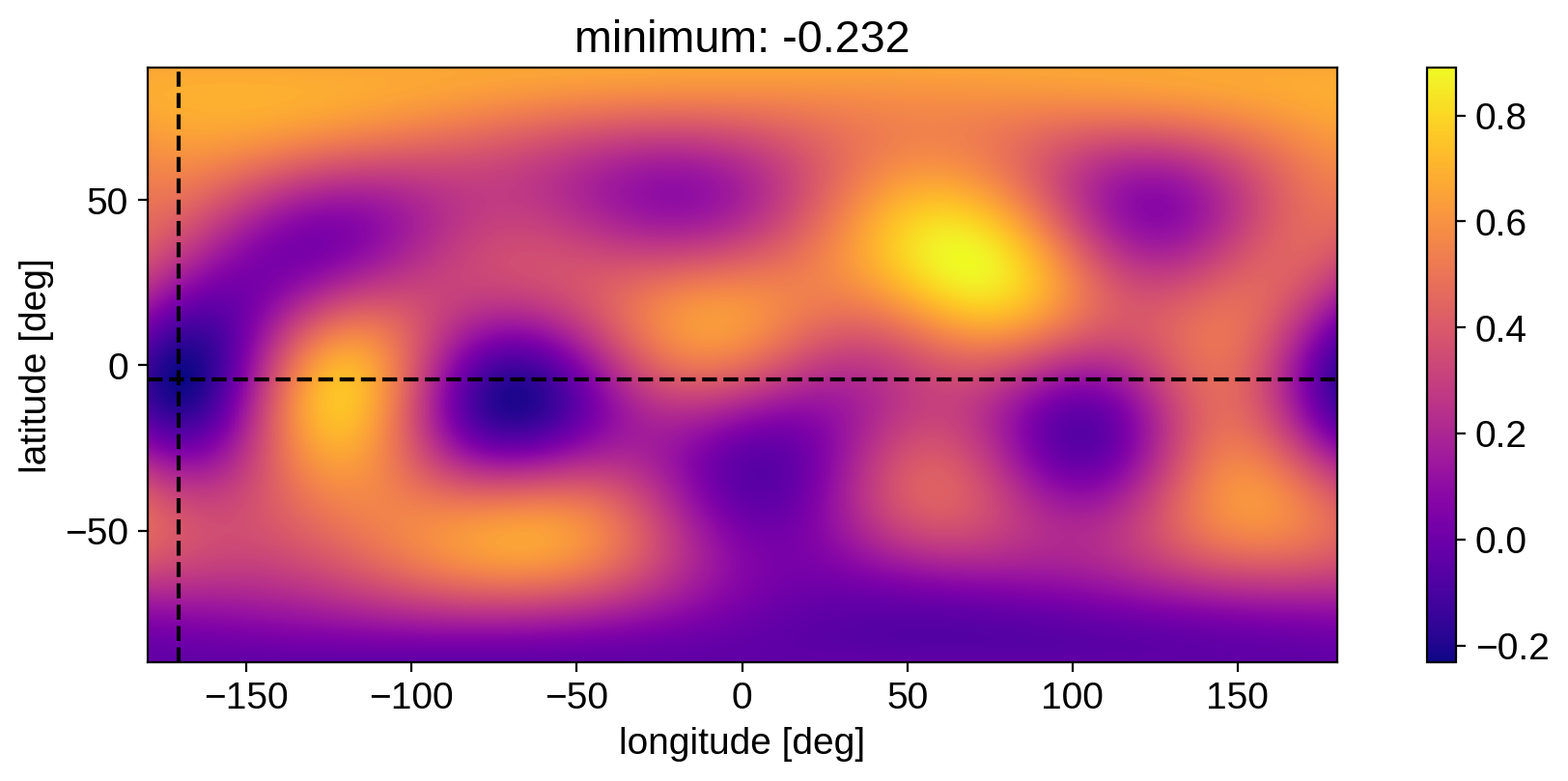
The method is fairly fast, so it could be used, for example, as a penalty when doing inference.

Limb-darkened maps

For limb-darkened maps, it’s a little easier to check whether the map is positive everywhere. Because the limb darkening profile is one-dimensional, we can use Sturm’s theorem to verify that

• The intensity is non-negative everywhere

• The intensity is monotonically decreasing toward the limb

Limb-darkened maps (or spherical harmonic maps with a limb darkening filter) implement the limbdark_is_physical method, which checks whether both points are true. Note, importantly, that the second point is specific to limb darkening. In principle the specific intensity could get brighter toward the limb (as is the case at certain wavelengths for the Sun), so you wouldn’t want to use in those cases.

map = starry.Map(udeg=4)

Let’s try this on a few limb-darkened maps:

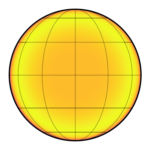
map[1:] = [0.5, 0.25, 0.5, 0.25]

map.show()

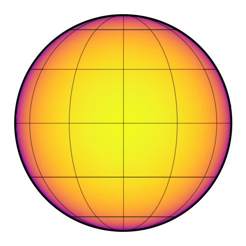
Is it physical?

map.limbdark_is_physical()

False

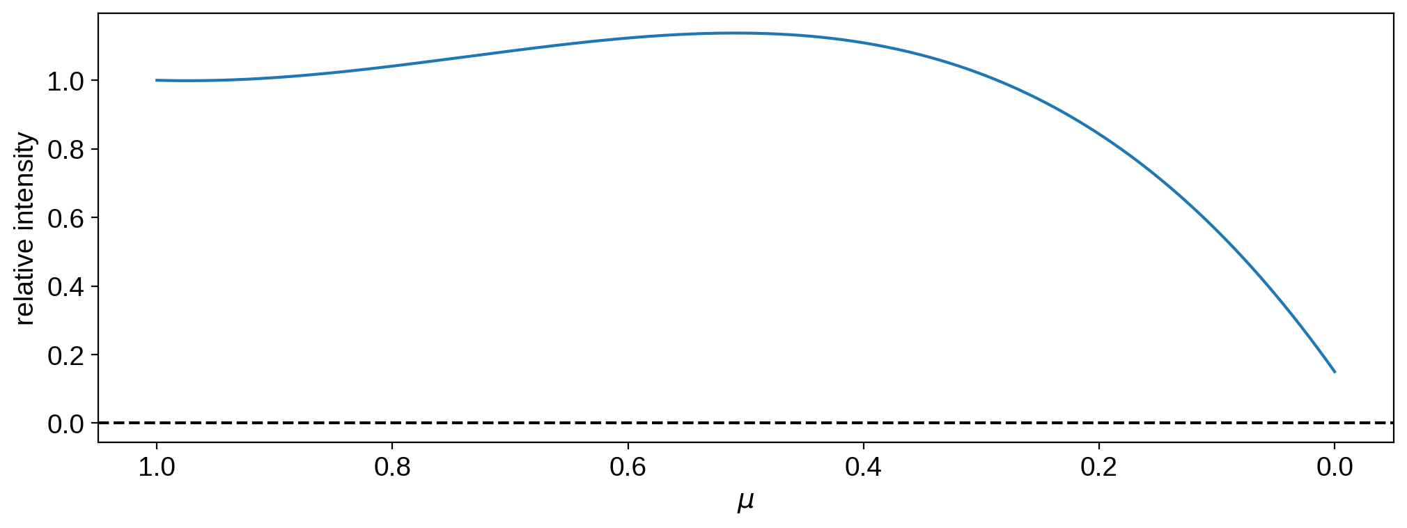
No! Let’s plot the intensity as a function of \(\mu\) to see why:

mu = np.linspace(0, 1, 1000)
plt.plot(mu, map.intensity(mu=mu))
plt.axhline(0, color="k", ls="--")
plt.gca().invert_xaxis()
plt.xlabel(r"$\mu$")
plt.ylabel("relative intensity");

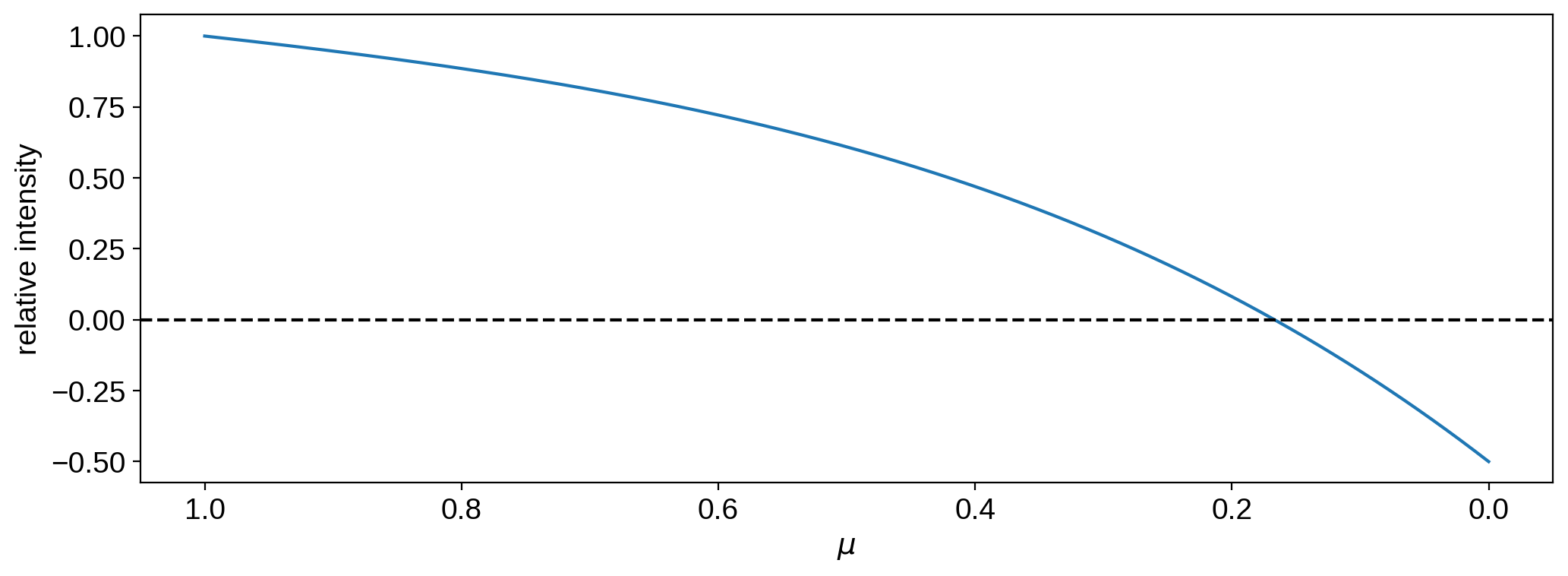
The intensity is negative close to the limb.

Let’s try a different coefficient vector:

map[1:] = [0.1, -2.0, 2.25, 0.5]

map.show()

Is it physical?

map.limbdark_is_physical()

False

mu = np.linspace(0, 1, 1000)
plt.plot(mu, map.intensity(mu=mu))
plt.axhline(0, color="k", ls="--")
plt.gca().invert_xaxis()
plt.xlabel(r"$\mu$")
plt.ylabel("relative intensity");

Even though it’s positive everywhere, it’s not monotonic!

One last example:

map[1:] = [0.5, -0.1, 0.25, 0.25]

map.show()

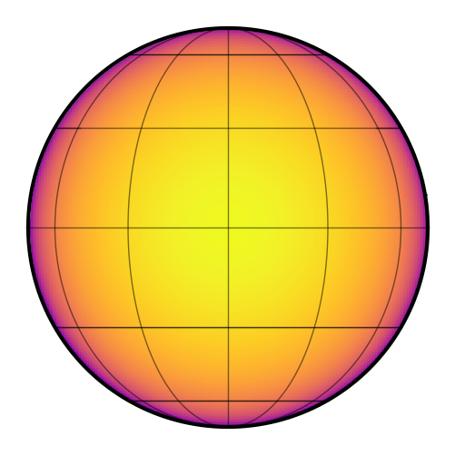
Is it physical?

map.limbdark_is_physical()

True

mu = np.linspace(0, 1, 1000)
plt.plot(mu, map.intensity(mu=mu))
plt.axhline(0, color="k", ls="--")
plt.gca().invert_xaxis()
plt.xlabel(r"$\mu$")
plt.ylabel("relative intensity");

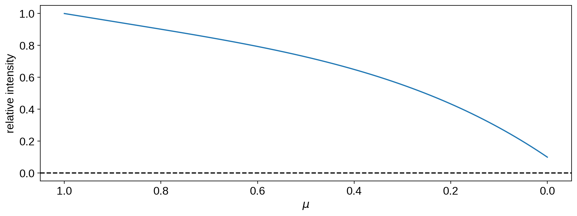
This one is both non-negative everywhere and monotonic, so it’s a physical limb darkening model.