Note

This tutorial was generated from a Jupyter notebook that can be downloaded here.

Star spots

A major part of the philosophy of starry is a certain amount of agnosticism about what the surface of a star or planet actually looks like. Many codes fit stellar light curves by solving for the number, location, size, and contrast of star spots. This is usually fine if you know the stellar surface consists of a certain number of discrete star spots of a given shape. In general, however, that’s a very strong prior to assume. And even in cases where it holds, the problem is still extremely degenerate and lies in a space that is quite difficult to sample.

Instead, in starry we assume the surface is described by a vector of spherical harmonic coefficients. The advantage of this is that (1) it automatically bakes in a Gaussian-process smoothness prior over the surface map, in which the scale of features is dictated by the degree of the expansion; and (2) under gaussian priors and gaussian errors, the posterior over surface maps is analytic. If and only if the data and prior support the existence of discrete star spots on the surface, the posterior will reflect that.

However, sometimes it’s convenient to restrict ourselves to the case of discrete star spots. In starry, we therefore implement the spot method, which adds a spot-like feature to the surface by expanding a circular top-hat in terms of spherical harmonics.

Note

This method replaced the add_spot method introduced in version 1.0.0.

In this notebook, we’ll take a look at how this new method works. For reference, here is the docstring of starry.Map.spot:

spot ( contrast=1.0, radius=None, lat=0.0, lon=0.0 )

Add the expansion of a circular spot to the map.

This function adds a spot whose functional form is a top hat in \(\Delta\theta\), the angular separation between the center of the spot and another point on the surface. The spot intensity is controlled by the parameter contrast, defined as the fractional change in the intensity at the center of the spot.

Parameters

• contrast (scalar or vector, optional) – The contrast of the spot. This is equal to the fractional change in the intensity of the map at the center of the spot relative to the baseline intensity of an unspotted map. If the map has more than one wavelength bin, this must be a vector of length equal to the number of wavelength bins. Positive values of the contrast result in dark spots; negative values result in bright spots. Default is 1.0, corresponding to a spot with central intensity close to zero.

• radius (scalar, optional) – The angular radius of the spot in units of angle_unit Defaults to 20.0 degrees.

• lat (scalar, optional) – The latitude of the spot in units of angle_unit Defaults to 20.0 degrees.

• lon (scalar, optional) – The longitude of the spot in units of angle_unit Defaults to 20.0 degrees.

Note

Keep in mind that things are normalized in starry such that the disk-integrated flux (not the intensity!) of an unspotted body is unity. The default intensity of an unspotted map is 1.0 / np.pi everywhere (this ensures the integral over the unit disk is unity). So when you instantiate a map and add a spot of contrast c, you’ll see that the intensity at the center is actually (1 - c) / np.pi. This is expected behavior, since that’s a factor of 1 - c smaller than the baseline intensity.

Note

This function computes the spherical harmonic expansion of a circular spot with uniform contrast. At finite spherical harmonic degree, this will return an approximation that may be subject to ringing. Users can control the amount of ringing and the smoothness of the spot profile (see below). In general, however, at a given spherical harmonic degree ydeg, there is always minimum spot radius that can be modeled well. For ydeg = 15, for instance, that radius is about 10 degrees. Attempting to add a spot smaller than this will in general result in a large amount of ringing and a smaller contrast than desired.

There are a few additional under-the-hood keywords that control the behavior of the spot expansion. These are

Parameters

• spot_pts (int, optional) – The number of points in the expansion of the (1-dimensional) spot profile. Default is 1000.

• spot_eps (float, optional) – Regularization parameter in the expansion. Default is 1e-9.

• spot_smoothing (float, optional) – Standard deviation of the Gaussian smoothing applied to the spot to suppress ringing (unitless). Default is 2.0 / self.ydeg.

• spot_fac (float, optional) – Parameter controlling the smoothness of the spot profile. Increasing this parameter increases the steepness of the profile (which approaches a top hat as spot_fac -> inf ). Decreasing it results in a smoother sigmoidal function. Default is 300. Changing this parameter is not recommended; change spot_smoothing instead.

Note

These last four parameters are cached. That means that changing their value in a call to spot will result in all future calls to spot “remembering” those settings, unless you change them back!

Adding a simple spot

Let’s begin by importing stuff as usual:

import numpy as np
import starry

starry.config.lazy = False
starry.config.quiet = True

The first thing we’ll do is create a dummy featureless map, which we’ll use for comparisons below.

map0 = starry.Map(ydeg=1)
map0.show()

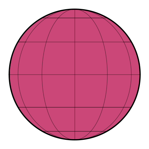
Now let’s instantiate a very high degree map and add a spot with a contrast of \(25\%\) and a radius of \(15^\circ\) at latitude/longitude \((0, 0)\):

contrast = 0.25
radius = 15
map = starry.Map(ydeg=30)
map.spot(contrast=contrast, radius=radius)

Here’s what we get:

map.show(theta=np.linspace(0, 360, 50))

The spot contrast

Let’s look at what a contrast of \(25\%\) implies for the actual intensity of points on the surface of our map. Fore definiteness, let’s look at the intensity along the equator:

lon = np.linspace(-90, 90, 100)
plt.plot(lon, map.intensity(lon=lon))
plt.xlabel("longitude [deg]")
plt.ylabel("intensity");

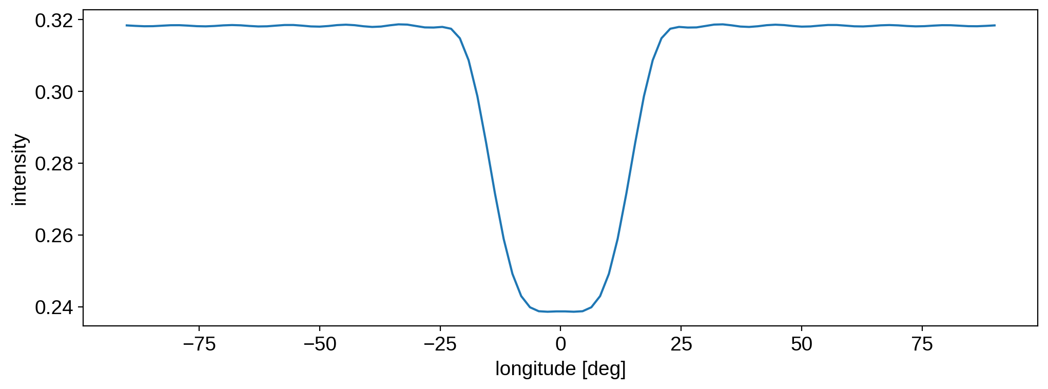
It’s worth recalling how intensities are normalized in starry (see the note in the docstring above). The baseline intensity of an unspotted map is 1.0 / np.pi, so the spot intensity is a \(25\%\) reduction relative to that value. Let’s normalize the function above to the continuum level to see that:

plt.plot(lon, np.pi * map.intensity(lon=lon))
plt.xlabel("longitude [deg]")
plt.ylabel("normalized intensity");

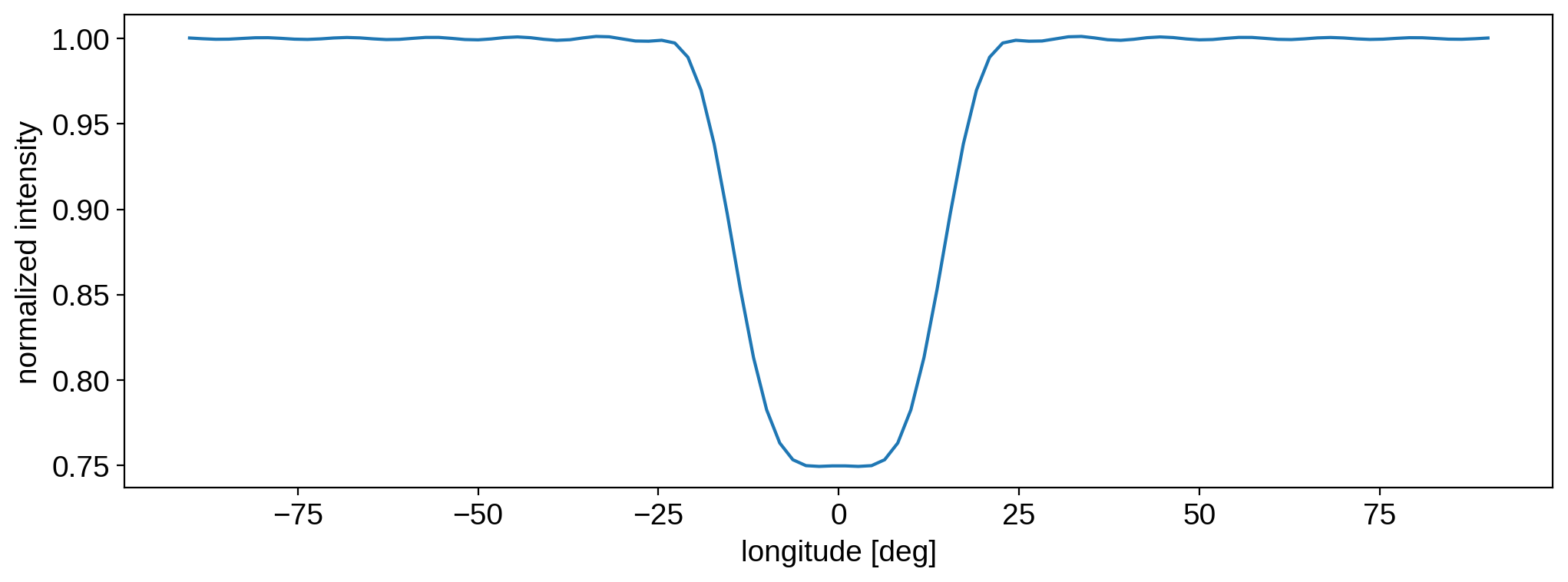
As expected, the intensity of the spot is \(25\%\) lower than the baseline.

The spot expansion

As mentioned in the docstring, the spot is modeled as a top hat in \(\Delta\theta\), the angular distance along the surface of the body. The profile in the figure above doesn’t really look like a top hat\(-\)that’s because we’re actually expanding the functional form of a top hat in the spherical harmonic basis. Since we’re at finite spherical harmonic degree, the expansion is not exact. In particular, the spherical harmonic basis enforces smoothing at small scales. You get the same behavior as if you tried to fit a 1d top hat with a low-order polynomial.

Because of this, there are a few things we must keep in mind.

First, the function we’re actually expanding is a sigmoid

\[f(\Delta\theta) = \frac{1}{1 + \exp \left( -c \Delta \theta \right)}\]

with smoothing parameter \(c\). In the limit that \(c \rightarrow \infty\), \(f(\Delta\theta)\) approaches an actual top hat. In practice, this can be problematic because of the discontinuity at \(\Delta\theta = r\), where the function is not differentiable. Setting \(c\) to a large but finite value makes the function continuous and differentiable everywhere.

Here’s the function we’re expanding for different values of \(c\):

radius = 15
dtheta = np.abs(lon) - radius
for c in [0.25, 0.5, 1, 10, 300]:
    plt.plot(lon, 1 / (1 + np.exp(-c * dtheta)), label=c)
plt.legend(title="c", fontsize=10)
plt.xlabel("angular distance [deg]")
plt.ylabel("intensity");

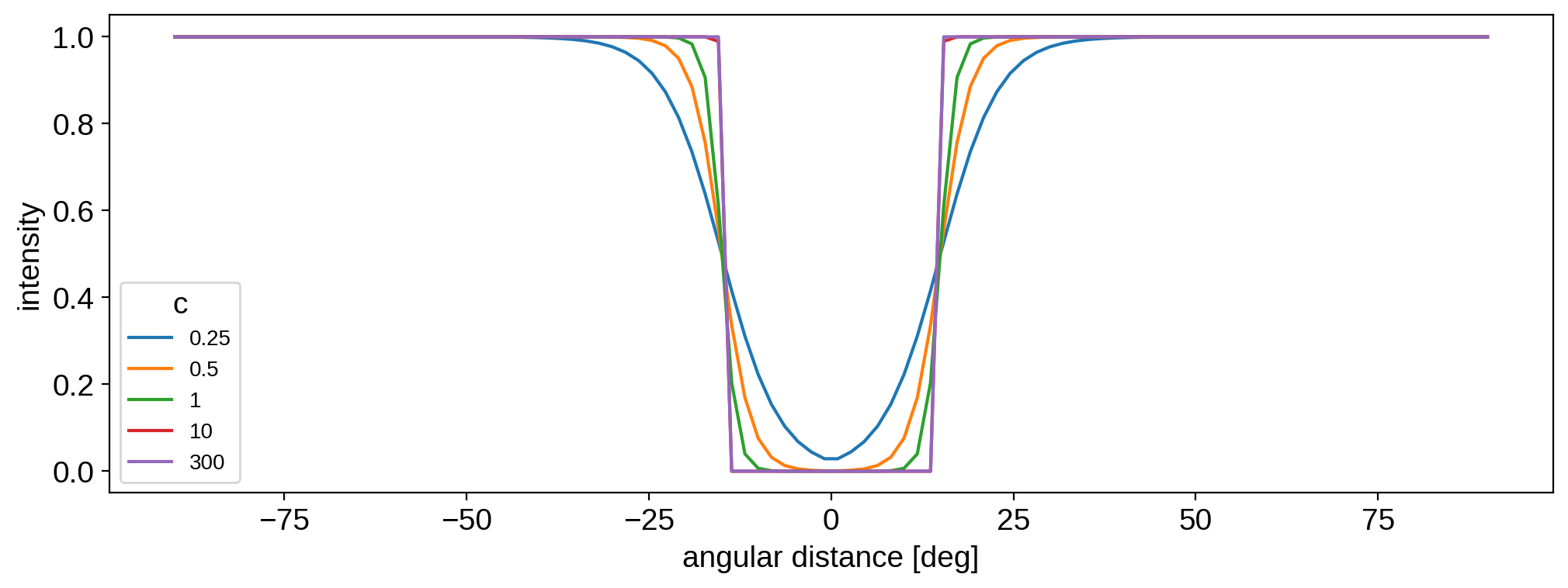
In starry, the smoothing parameter \(c\) is specified as the keyword spot_fac (see docs above). By default it’s set to 300 (purple line), so it’s actually almost indistinguishable from a true top hat.

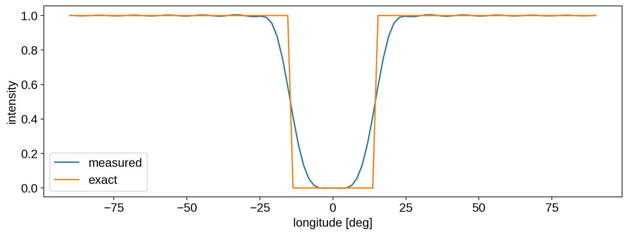
OK, but even though the function we’re expanding is almost exactly a top hat, the actual intensity on the surface of the sphere is much smoother. That’s because of the finite spherical harmonic expansion, as mentioned above. Let’s compare the input function and the actual intensity profile after the expansion:

# Plot the starry intensity along the equator
map.reset()
map.spot(contrast=1, radius=radius)
plt.plot(lon, np.pi * map.intensity(lon=lon), label="measured")

# Plot the actual function we're expanding
c = 300
dtheta = np.abs(lon) - radius
plt.plot(lon, 1 / (1 + np.exp(-c * dtheta)), label="exact")

plt.legend()
plt.xlabel("longitude [deg]")
plt.ylabel("intensity");

There’s actually another level of smoothing happening in starry that is controlled by the spot_smoothing parameter. Let’s look at what the measured intensity profile would be if we got rid of smoothing altogether:

# Plot the starry intensity along the equator
map.reset()
map.spot(contrast=1, radius=radius, spot_smoothing=0)
plt.plot(lon, np.pi * map.intensity(lon=lon), label="measured (no smoothing)")

# Plot the actual function we're expanding
c = 300
dtheta = np.abs(lon) - radius
plt.plot(lon, 1 / (1 + np.exp(-c * dtheta)), label="exact")

plt.legend()
plt.xlabel("longitude [deg]")
plt.ylabel("intensity");

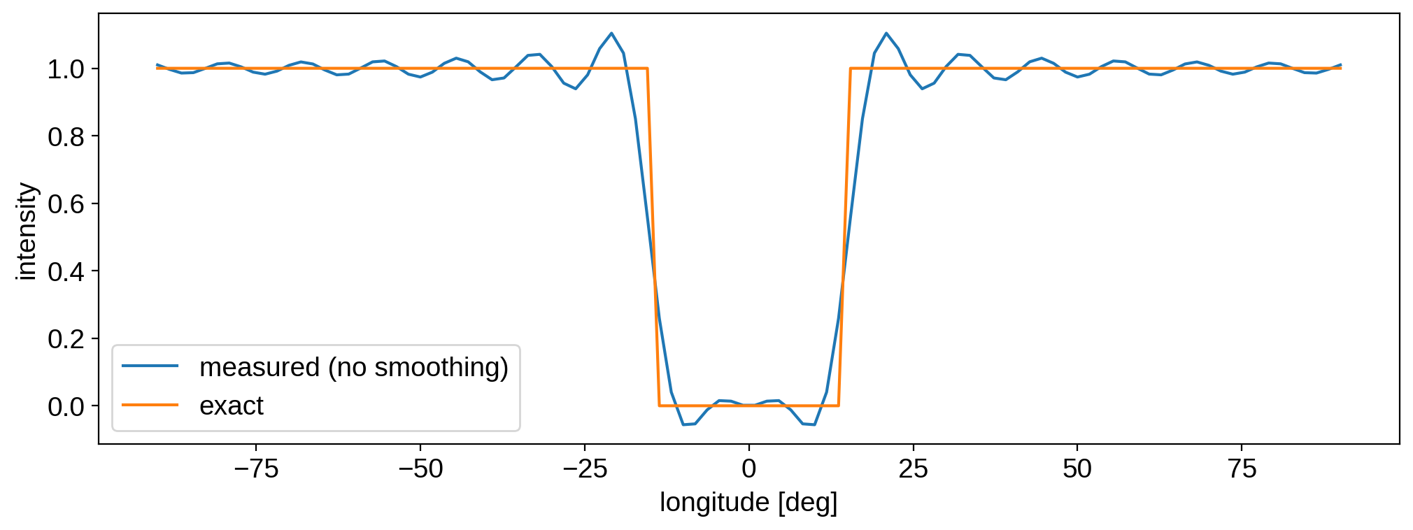
The measured intensity is steeper and closer to the exact profile at \(\Delta\theta = r\), but we’re paying a high price for this with all the ringing! This is the classical Gibbs phenomenon, which you’ve seen if you’ve ever tried to compute the Fourier expansion (or transform) of a square wave. At finite degree, the spherical harmonic basis simply can’t capture sharp discontinuities. The spot_smoothing parameter convolves the surface map with a function of the form

\[s(\sigma) = \exp\left(-l \left(l + 1\right) \sigma^2 \right)\]

where \(\sigma =\) spot_smoothing. By default, this is equal to 2 / self.ydeg, which results in the smooth (but gentler) spot profile in the previous figure. Increase this to suppress ringing, at the expense of a smoother profile; decrease it for the opposite effect.

The final point we should address concerns the minimum radius we can model at a given spherical harmonic degree. Let’s visualize the measured spot profile for different radii ranging from \(3^\circ\) to \(25^\circ\) (using the original, smoothed map):

lon = np.linspace(-45, 45, 300)
radii = np.arange(3, 26)
cmap = plt.get_cmap("plasma_r")
for k, radius in enumerate(radii):
    map.reset()
    map.spot(contrast=1, radius=radius, spot_smoothing=2 / map.ydeg)
    plt.plot(
        lon, np.pi * map.intensity(lon=lon), color=cmap(0.25 + 0.5 * k / len(radii))
    )
    if radius <= 10:
        plt.text(
            0, 0.01 + np.pi * map.intensity(lon=0), radius, ha="center", fontsize=6
        )
    if radius == 25:
        plt.text(
            0, -0.05 + np.pi * map.intensity(lon=0), radius, ha="center", fontsize=6
        )
plt.xlabel("longitude [deg]")
plt.ylabel("intensity");

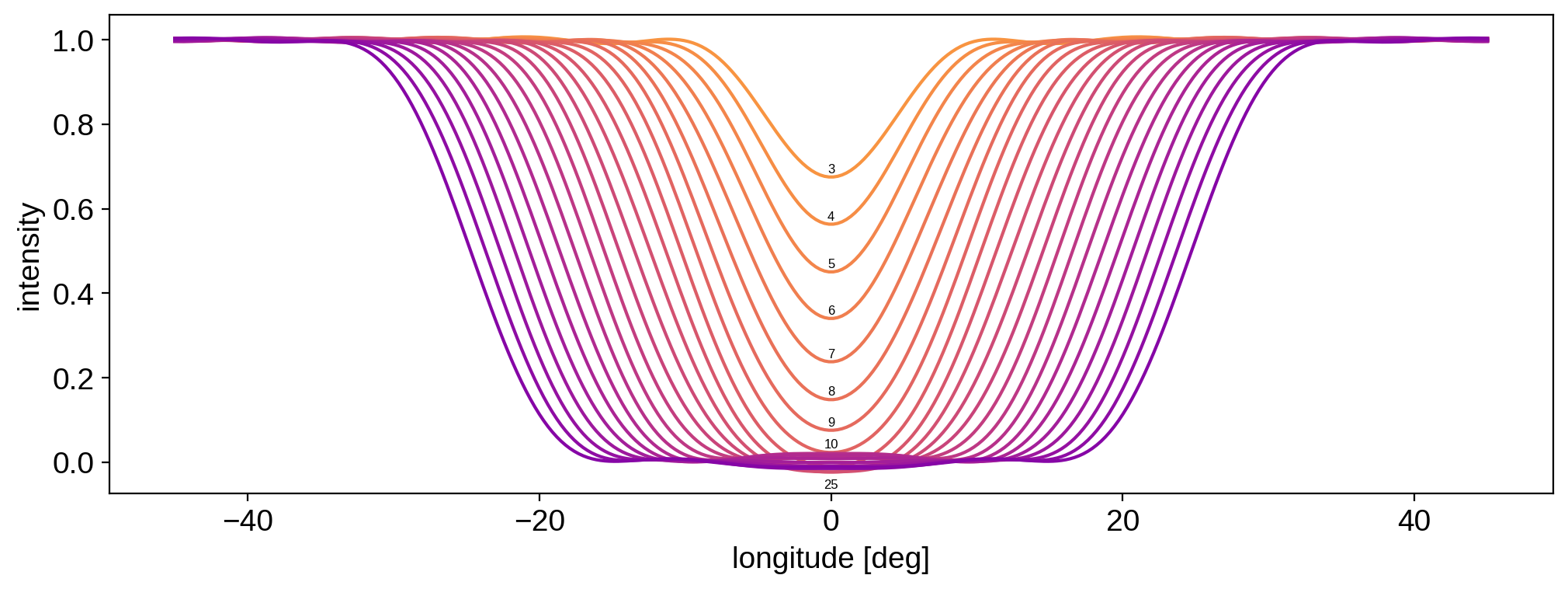
For \(r \ge 10^\circ\), the spherical harmonic expansion has no trouble in capturing the spot profile. But for smaller radii, the profile doesn’t actually get any smaller\(-\)instead, its amplitude starts to decrease! That’s because a spherical harmonic expansion of degree ydeg has a minimum angular scale it can model\(-\)below that scale, things get smoothed away (and their amplitude gets washed out). The angular scale is proportional to 1/ydeg. As a very rough rule of thumb, it scales as 180 / ydeg. That would mean our minimum diameter is \(6^\circ\) (or a radius of \(3^\circ\), but that doesn’t account for the fact that we are adding additional smoothing to suppress ringing. That smoothing makes the minimum radius closer to \(10^\circ\) for ydeg=30.

If we weren’t adding any smoothing, then we can see that the limiting radius is in fact very close to \(3^\circ\):

lon = np.linspace(-45, 45, 300)
radii = np.arange(3, 26)
cmap = plt.get_cmap("plasma_r")
for k, radius in enumerate(radii):
    map.reset()
    map.spot(contrast=1, radius=radius, spot_smoothing=0)
    plt.plot(
        lon, np.pi * map.intensity(lon=lon), color=cmap(0.25 + 0.5 * k / len(radii))
    )
    if radius == 3:
        plt.text(
            0, 0.01 + np.pi * map.intensity(lon=0), radius, ha="center", fontsize=6
        )
plt.xlabel("longitude [deg]")
plt.ylabel("intensity");

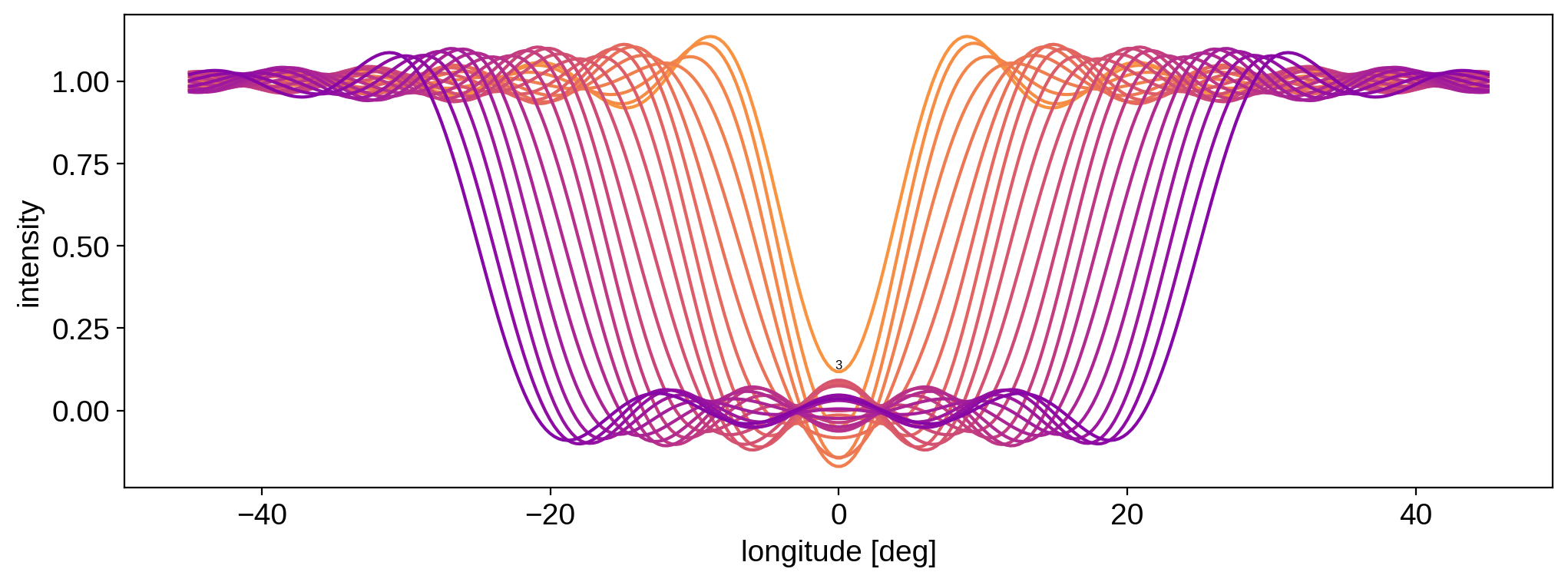
But in many cases, that may be an unacceptable level of ringing.

Long story short: there’s always going to be a trade-off between the amount of ringing and the maximum resolution of features you can model at a given spherical harmonic degree.

The last thing we’ll do in this tutorial is compute the minimum spot radius we can model at a given spherical harmonic degree and with a given smoothing strength. We’ll define this minimum value as the radius below which we get more than \(10\%\) error in the mean contrast of the spot. You can change this tolerance by tweaking the tol parameter below:

smstrs = [0.0, 1.0, 2.0]
ydegs = [10, 15, 20, 25, 30]
radii = np.arange(1, 90)
tol = 0.1
rmin = np.zeros((len(smstrs), len(ydegs)))
for i, smstr in enumerate(smstrs):
    for j, ydeg in enumerate(ydegs):
        map = starry.Map(ydeg)
        error = np.zeros(len(radii))
        for radius in radii:
            map.reset()
            map.spot(contrast=1, radius=radius, spot_smoothing=smstr / ydeg)
            if (
                np.abs(np.mean(map.intensity(lon=np.linspace(0, 0.75 * radius, 50))))
                < tol
            ):
                rmin[i, j] = radius
                break
plt.figure(figsize=(8, 8))
plt.plot(ydegs, rmin[0], "-o", label=r"$0$")
plt.plot(ydegs, rmin[1], "-o", label=r"$1 / l_\mathrm{max}$")
plt.plot(ydegs, rmin[2], "-o", label=r"$2 / l_\mathrm{max}$ (default)")
plt.legend(title="smoothing", fontsize=10)
plt.xticks([10, 15, 20, 25, 30])
plt.xlabel(r"spherical harmonic degree $l_\mathrm{max}$")
plt.ylabel(r"minimum spot radius [degrees]");

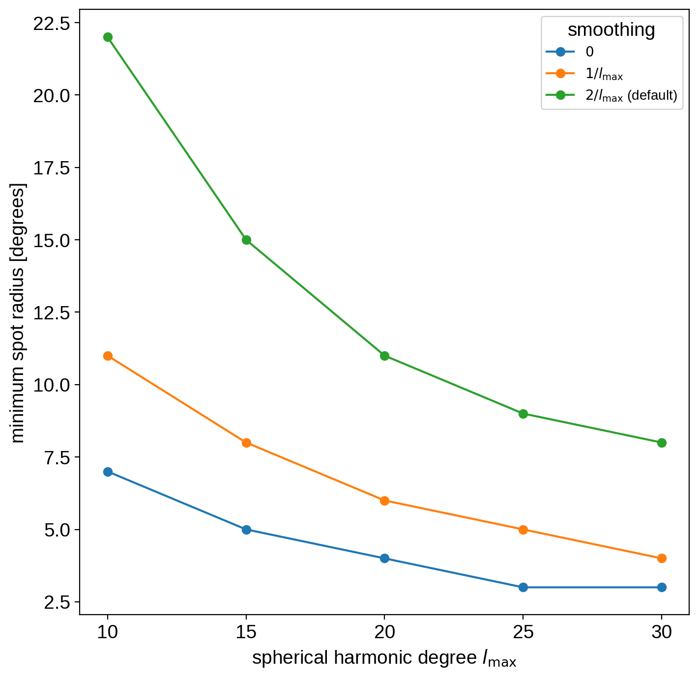
The green line shows the default smoothing strength (the spot_smoothing parameter); the orange line shows half that amount of smoothing, and the blue line shows no smoothing. In all cases, the minimum radius we can safely model decreases roughly as \(1/l_\mathrm{max}\).

Use this figure as a rule of thumb when modeling discrete spots with starry.