Note
This tutorial was generated from a Jupyter notebook that can be downloaded here.
Linear solve
In this notebook we discuss how to linearly solve for the posterior over spherical harmonic coefficients of a map given a light curve. This is similar to what we did in the Eclipsing Binary notebook. The idea is to take advantage of the linearity of the starry solution to analytically compute the posterior over maps consistent with the data.
[3]:
import matplotlib.pyplot as plt
import numpy as np
import starry

np.random.seed(12)
starry.config.lazy = False
starry.config.quiet = True
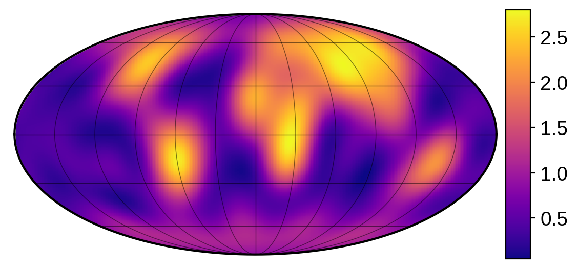
We’re going to demonstrate the linear solve feature using a map in reflected light, since the presence of a day/night terminator breaks many degeneracies and makes the mapping problem much less ill-posed. Let’s begin by instantiating a reflected light map of the Earth. We’ll give it the same obliquity as the Earth and observe it at an inclination of 60 degrees. We’ll also give it an amplitude of 0.16: this is the value that will scale the surface map everywhere, which
we can see leads to a continental albedo of about 0.4, which is (very) roughly what we expect for the Earth:
[4]:
map = starry.Map(ydeg=10, reflected=True)
map.load("earth", force_psd=True)
map.amp = 0.16
map.obl = 23.5
map.inc = 60
map.show(illuminate=False, colorbar=True, projection="moll")
Note
The force_psd keyword in load() forces the map to be positive semi-definite (PSD),
that is, it forces the albedo to be non-negative everywhere on the surface. Ensuring a
spherical harmonic expansion is PSD is not trivial; we do this numerically, so it takes
a little longer than if force_psd were False. It’s also not perfect, since the
numerical search for the map minimum is tricky. After it’s done, starry re-normalizes
the map so that minimum value is nudged to zero.
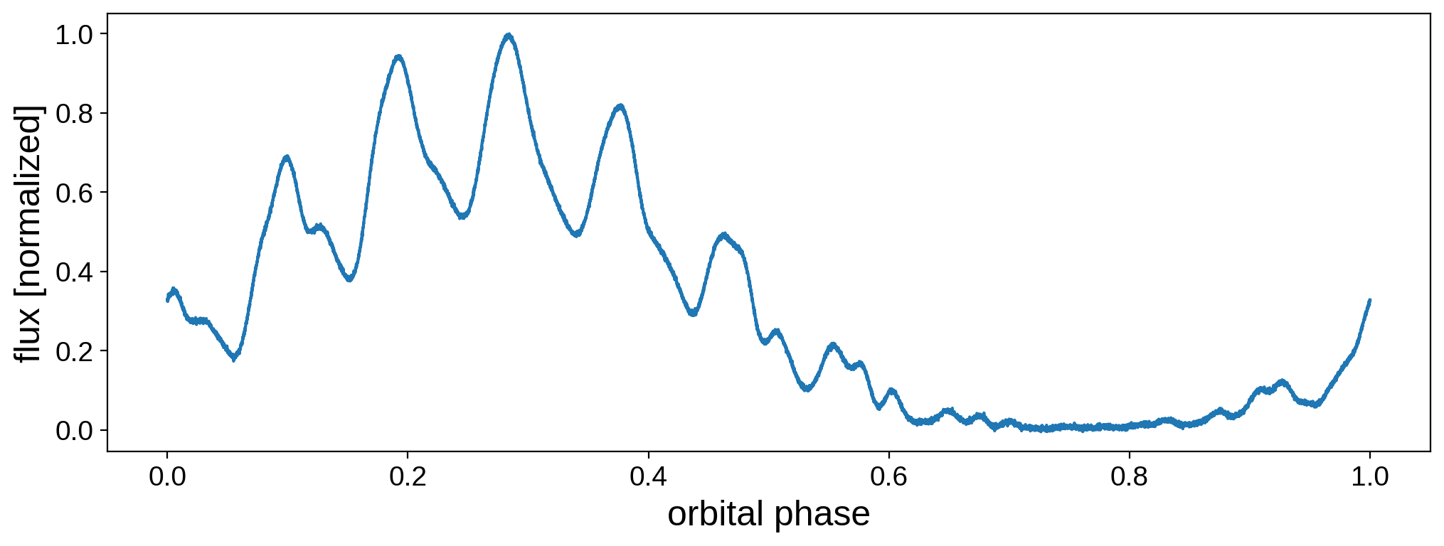
Now we generate a dataset. We’ll assume we have 10,000 observations over the course of a full orbit of the planet. We further take the planet’s rotation period to be one-tenth of its orbital period. This will give us good coverage during all seasons, maximizing the amount of data we have for all the different regions of the planet:
[5]:
# Make the planet rotate 10 times over one full orbit
npts = 10000
nrot = 10
time = np.linspace(0, 1, npts)
theta = np.linspace(0, 360 * nrot, npts)

# Position of the star relative to the planet in the orbital plane
t = np.reshape(time, (1, -1))
p = np.vstack((np.cos(2 * np.pi * t), np.sin(2 * np.pi * t), 0 * t))

# Rotate to an observer inclination of 60 degrees
ci = np.cos(map.inc * np.pi / 180)
si = np.sin(map.inc * np.pi / 180)
R = np.array([[1, 0, 0], [0, ci, -si], [0, si, ci]])
xs, ys, zs = R.dot(p)

# Keywords to the `flux` method
kwargs = dict(theta=theta, xs=xs, ys=ys, zs=zs)
[6]:
# Compute the flux
flux0 = map.flux(**kwargs)
sigma = 0.0005
flux = flux0 + sigma * np.random.randn(npts)

# Normalize it to a maximumm of unity
flux /= np.max(flux)
[7]:
fig, ax = plt.subplots(1, figsize=(12, 4))
ax.plot(time, flux)
ax.set_xlabel("orbital phase", fontsize=18)
ax.set_ylabel("flux [normalized]", fontsize=18);
Now the fun part. Let’s instantiate a new map so we can do inference on this dataset:
[8]:
map = starry.Map(ydeg=10, reflected=True)
map.obl = 23.5
map.inc = 60
We now set the data vector (the flux and the covariance matrix):
[9]:
map.set_data(flux, C=sigma ** 2)
And now the prior, which is also described as a multivariate gaussian with a mean \(\mu\) and covariance \(\Lambda\). This is the prior on the amplitude-weighted spherical harmonic coefficients. In other words, if \(\alpha\) is the map amplitude (map.amp) and \(y\) is the vector of spherical harmonic coefficients (map.y), we are placing a prior on the quantity \(x \equiv \alpha y\). While this may be confusing at first, recall that the coefficient of the
\(Y_{0,0}\) harmonic is fixed at unity in starry, so we can’t really solve for it. But we can solve for all elements of the vector \(x\). Once we have the posterior for \(x\), we can easily obtain both the amplitude (equal to \(x_0\)) and the spherical harmonic coefficient vector (equal to \(x / x_0\)). This allows us to simultaneously obtain both the amplitude and the coefficients using a single efficient linear solve.
For the mean \(\mu\), we’ll set the first coefficient to unity (since we expect \(\alpha\) to be distributed somewhere around one, if the light curve is properly normalized) and all the others to zero (since our prior is isotropic and we want to enforce some regularization to keep the coefficients small).
For the covariance \(\Lambda\) (L in the code), we’ll make it a diagonal matrix. The first diagonal entry is the prior variance on the amplitude of the map, and we’ll set that to \(1\). The remaining entries are the prior variance on the amplitude-weighted coefficients. We’ll pick something small – \(10^{-5}\)– to keep things well regularized. In practice, this prior is related to our beliefs about the angular power spectrum of the map.
[10]:
mu = np.empty(map.Ny)
mu[0] = 1
mu[1:] = 0
L = np.empty(map.Ny)
L[0] = 1e0
L[1:] = 1e-5
map.set_prior(L=L)
Finally, we call solve, passing in the kwargs from before. In this case, we’re assuming we know the orbital information exactly. (When this is not the case, we need to do sampling for the orbital parameters; we cover this in more detail in the Eclipsing Binary tutorial).
[11]:
%%time
mu, cho_cov = map.solve(**kwargs)
CPU times: user 524 ms, sys: 128 ms, total: 652 ms
Wall time: 3.01 s
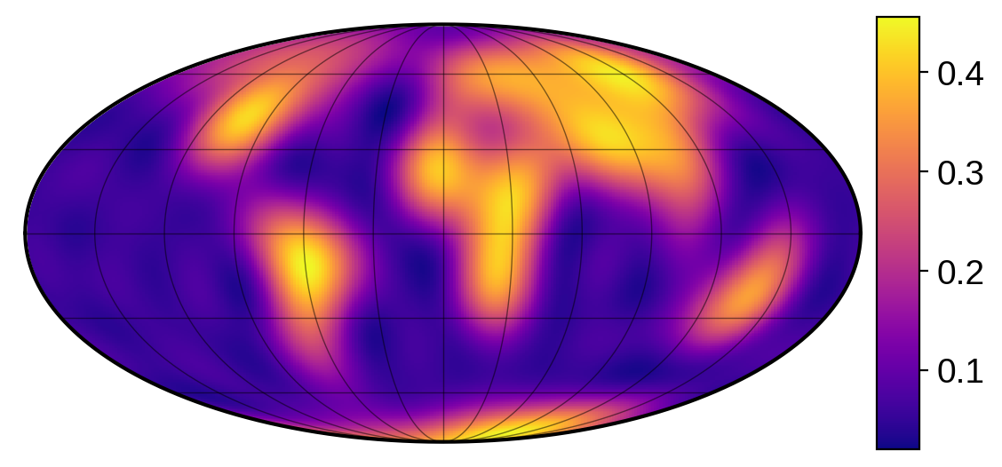
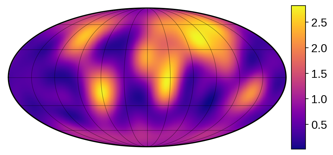
The solve method sets the map coefficicents to the maximum a posteriori (MAP) solution. Let’s view this mean map:
[12]:
map.show(illuminate=False, colorbar=True, projection="moll")
Note that the normalization is different (unphysical even!), but that’s only because we normalized our flux vector. Because we divided out the maximum flux, there’s nothing in the data telling us what the actual albedo of the surface is. (When modeling a real dataset, if we knew the distance from the planet to the star and modelled the flux in real units, we could easily fix this).
We can also draw a random sample from the posterior (which automatically sets the map amplitude and coefficients) by calling
[13]:
np.random.seed(3)
map.draw()
[14]:
map.show(illuminate=False, colorbar=True, projection="moll")
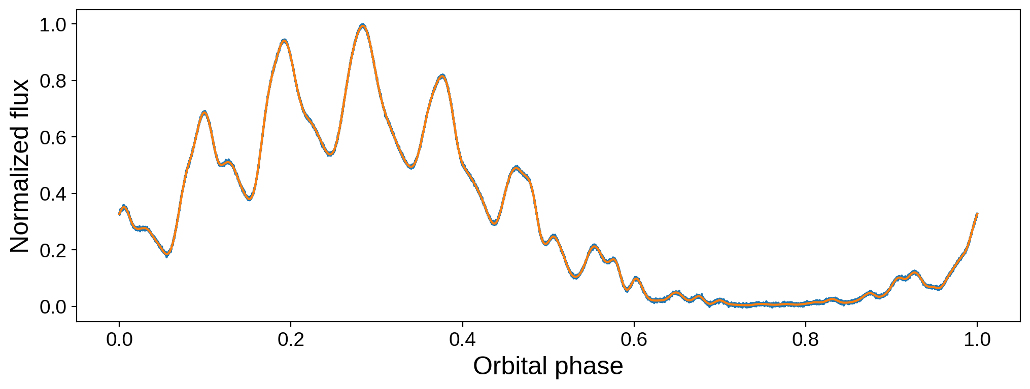
We can verify that we got a good fit to the data from this random sample:
[15]:
fig, ax = plt.subplots(1, figsize=(12, 4))
ax.plot(time, flux)
plt.plot(time, map.flux(**kwargs))
ax.set_xlabel("Orbital phase", fontsize=18)
ax.set_ylabel("Normalized flux", fontsize=18);