Note
This tutorial was generated from a Jupyter notebook that can be downloaded here.
The basics
Here we’ll discuss how to instantiate spherical harmonic maps, manipulate them, plot them, and compute simple phase curves and occultation light curves.
Introduction
Surface maps in starry are described by a vector of spherical harmonic coefficients. Just like polynomials on the real number line, spherical harmonics form a complete basis on the surface of the sphere. Any surface map can be expressed as a linear combination of spherical harmonics, provided one goes to sufficiently high degree in the expansion.
In starry, the surface map is described by the vector y, which is indexed by increasing degree \(l\) and order \(m\):
\(y = \{Y_{0,0}, \, Y_{1,-1}, \, Y_{1,0}, \, Y_{1,1} \, Y_{2,-2}, \, Y_{2,-1}, \, Y_{2,0} \, Y_{2,1}, \, Y_{2,2}, \, ...\}\).
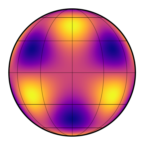
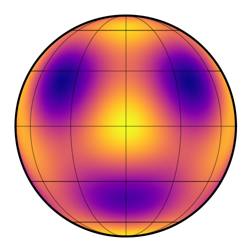
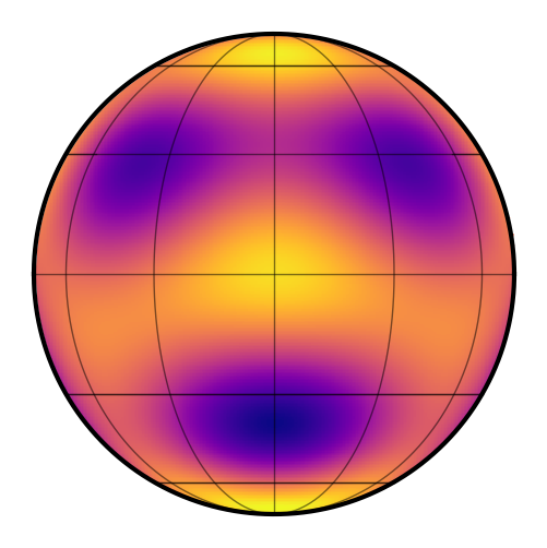
For reference, here’s what the first several spherical harmonic degrees look like:
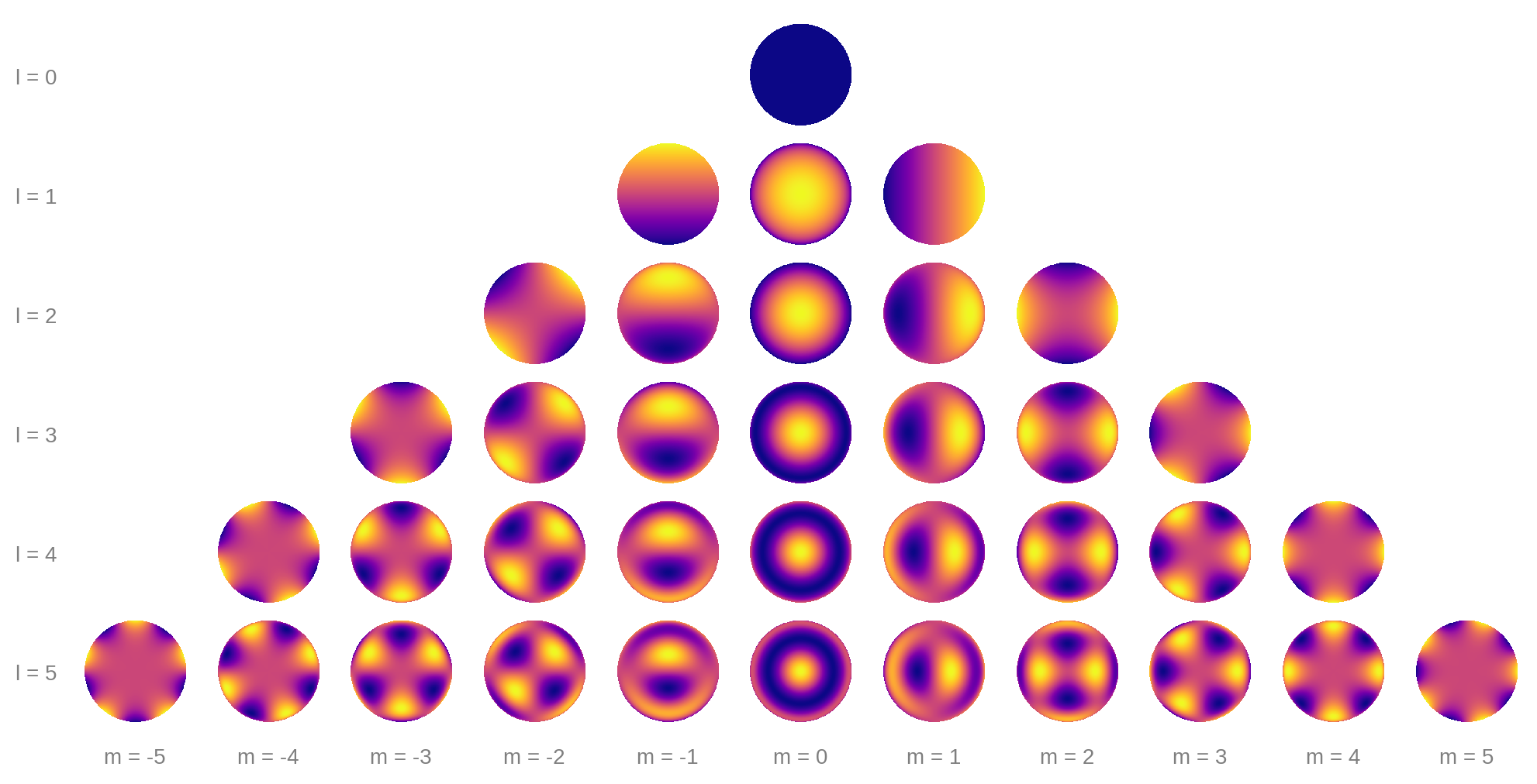
Each row corresponds to a different degree \(l\), starting at \(l = 0\). Within each row, the harmonics extend from order \(m = -l\) to order \(m = l\).
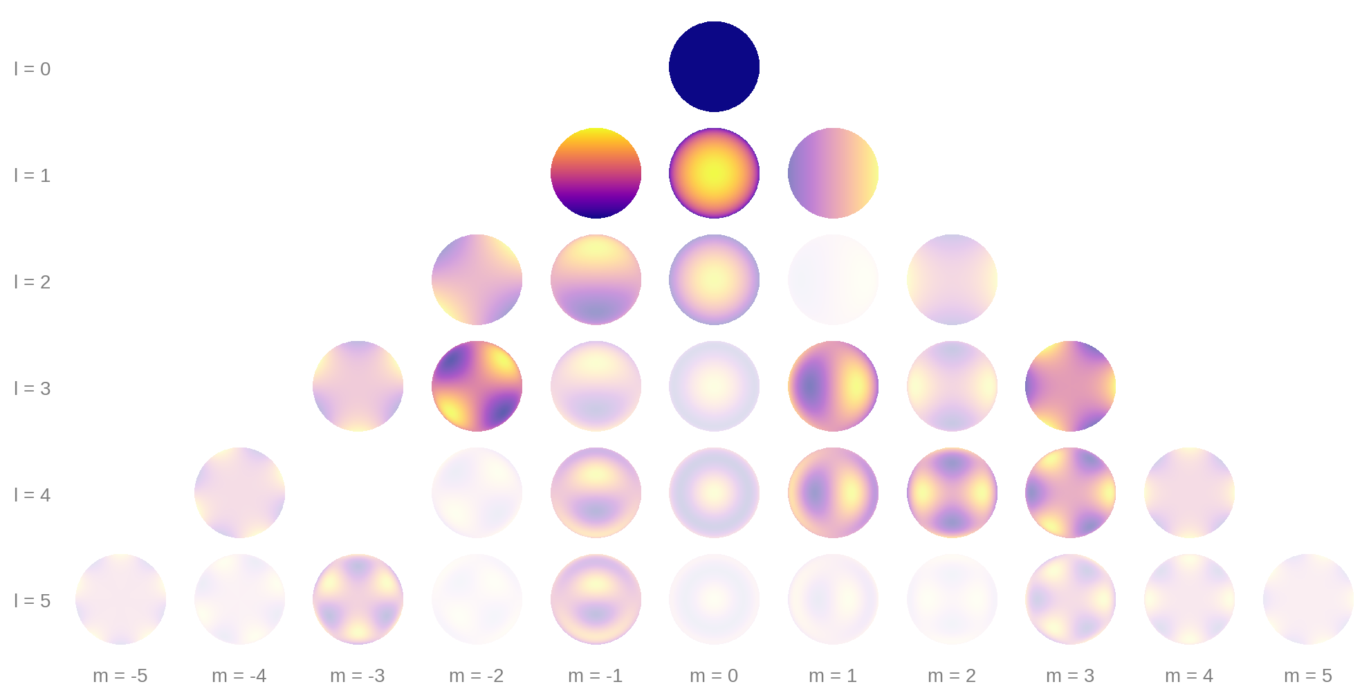
As an example, suppose we have the following map vector:
y = [1.00,  0.22,  0.19,  0.11,  0.11,  0.07,  -0.11, 0.00,  -0.05,
     0.12,  0.16,  -0.05, 0.06,  0.12,  0.05,  -0.10, 0.04,  -0.02,
     0.01,  0.10,  0.08,  0.15,  0.13,  -0.11, -0.07, -0.14, 0.06,
     -0.19, -0.02, 0.07,  -0.02, 0.07,  -0.01, -0.07, 0.04,  0.00]
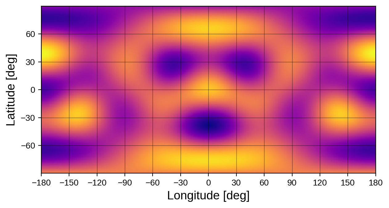
This is how much each spherical harmonic is contributing to the sum:
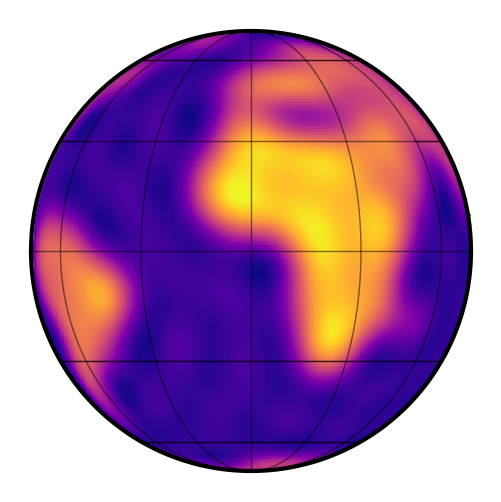
If we add up all of the terms, we get the following image:
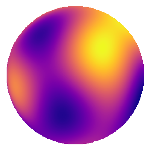
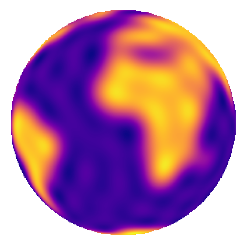
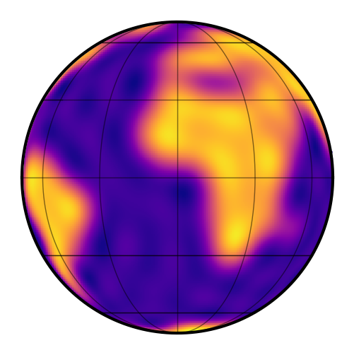
which is the \(l = 5\) spherical harmonic expansion of a map of the Earth! South America is to the left and Africa is toward the top right. It might still be hard to see, so here’s what we would get if we carried the expansion up to degree \(l = 20\):
Using starry
OK, now that we’ve introduced the spherical harmonics, let’s look at how we can use starry to model some celestial bodies.
The first thing we should do is import starry and instantiate a Map object. This is the simplest way of creating a spherical harmonic map. The Map object takes a few arguments, the most important of which is ydeg, the highest degree of the spherical harmonics used to describe the map. Let’s create a fifth-degree map:
[8]:
import starry

starry.config.lazy = False

map = starry.Map(ydeg=5)
(We’re disabling lazy evaluation in this notebook; see here for more details.) The y attribute of the map stores the spherical harmonic coefficients. We can see that our map is initialized to a constant map:
[9]:
map.y
[9]:
array([1., 0., 0., 0., 0., 0., 0., 0., 0., 0., 0., 0., 0., 0., 0., 0., 0.,
       0., 0., 0., 0., 0., 0., 0., 0., 0., 0., 0., 0., 0., 0., 0., 0., 0.,
       0., 0.])
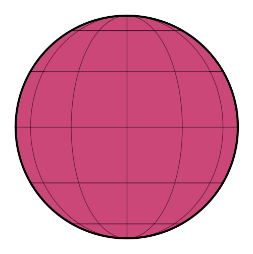
The \(Y_{0,0}\) coefficient is always fixed at unity, and by default all other coefficients are set to zero. Our map is therefore just the first spherical harmonic, which if you scroll up you’ll see is that constant dark blue disk at the top of the first figure. We can also quickly visualize the map by calling the show method:
[10]:
map.show()
Not that interesting! But before we give this map some features, let’s briefly discuss how we would evaluate our map. This means computing the intensity at a latitude/longitude point on the surface. Let’s investigate the intensity at the center (lat = lon = 0) of the map:
[11]:
map.intensity(lat=0, lon=0)
[11]:
array([0.31830989])
Since our map is constant, this is the intensity everywhere on the surface. It may seem like a strange number, but perhaps it will make sense if compute what the total flux (intensity integrated over area) of the map is. Since the map is constant, and since the body we’re modeling has unit radius by default, the total flux visible to the observer is just…
[12]:
import numpy as np

np.pi * 1.0 ** 2 * map.intensity(lat=0, lon=0)
[12]:
array([1.])
So the total flux visible from the map is unity. This is how maps in starry are normalized: the average disk-integrated intensity is equal to the coefficient of the constant \(Y_{0,0}\) harmonic, which is fixed at unity. We’re going to discuss in detail how to compute fluxes below, but here’s a sneak peek:
[13]:
map.flux()
[13]:
array([1.])
Given zero arguments, the flux method of the map returns the total visible flux from the map, which as we showed above, is just unity.
Setting map coefficients
Okay, onto more interesting things. Setting spherical harmonic coefficients is extremely easy: we can assign values directly to the map instance itself. Say we wish to set the coefficient of the spherical harmonic \(Y_{5, -3}\) to \(-2\). We simply run
[14]:
map[5, -3] = -2
We can check that the spherical harmonic vector (which is a flattened version of the image we showed above) has been updated accordingly:
[15]:
map.y
[15]:
array([ 1.,  0.,  0.,  0.,  0.,  0.,  0.,  0.,  0.,  0.,  0.,  0.,  0.,
        0.,  0.,  0.,  0.,  0.,  0.,  0.,  0.,  0.,  0.,  0.,  0.,  0.,
        0., -2.,  0.,  0.,  0.,  0.,  0.,  0.,  0.,  0.])
And here’s what our map now looks like:
[16]:
map.show()
Just for fun, let’s set two additional coefficients:
[17]:
map[5, 0] = 2
map[5, 4] = 1
[18]:
map.show()
Kind of looks like a smiley face!
Pro tip: To turn your smiley face into a Teenage Mutant Ninja Turtle, simply edit the \(Y_{5,2}\) coefficient:
[19]:
map[5, 2] = 1.5
map.show()
It’s probably useful to play around with setting coefficients and plotting the resulting map to get a feel for how the spherical harmonics work.
Two quick notes on visualizing maps: first, you can animate them by passing a vector theta argument to show(); this is just the rotational phase at which the map is viewed. By default, angles in starry are in degrees (this can be changed by setting map.angle_unit).
[20]:
theta = np.linspace(0, 360, 50)
map.show(theta=theta)
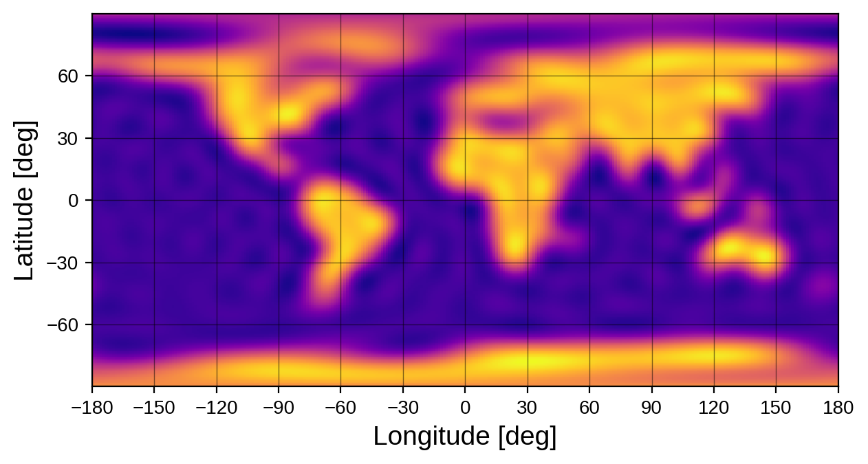
Second, we can easily get an equirectangular (latitude-longitude) global view of the map as follows:
[21]:
map.show(projection="rect")
Loading map images
In addition to directly specifying the spherical harmonic coefficients of a map, users can “load” images into starry via the load() method, which computes the spherical harmonic expansion of whatever image/array is provided to it. Users can pass paths to image files, numpy arrays on a rectangular latitude/longitude grid, or Healpix maps. starry comes with a few built-in maps to play around with:
Let’s load the earth map and see what we get:
[23]:
map = starry.Map(ydeg=20)
map.load("earth", sigma=0.08)
map.show()
[24]:
map.show(projection="rect")
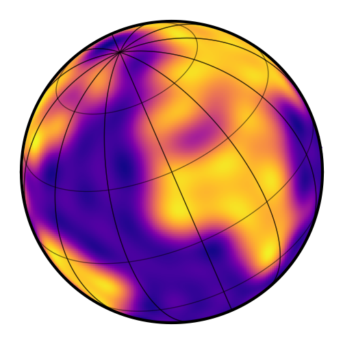
Changing the orientation
We can change the orientation of the map by specifying its inclination inc and obliquity obl. Note that these are properties of the observer. Changing these values changes the vantage point from which we see the map; it does not change the internal spherical harmonic representation of the map. Rather, map coefficients are defined in a static, invariant frame and the map can be observed from different vantage points by changing these angles. (This is different from the convention in
version 0.3.0 of the code; see the tutorial on Map Orientation for more information).
The obliquity is measured as the rotation angle of the objecet on the sky plane, measured counter-clockwise from north. The inclination is measured as the rotation of the object away from the line of sight. Let’s set the inclination and obliquity of the Earth as an example:
[25]:
map.obl = 23.5
map.inc = 60.0
map.show()
Computing the intensity
We already hinted at how to compute the intensity at a point on the surface of the map: just use the intensity() method. This method takes the latitude and longitude of a point or a set of points on the surface and returns the specific intensity at each one.
As an example, let’s plot the intensity of the Earth along the equator:
[26]:
lon = np.linspace(-180, 180, 1000)
I = map.intensity(lat=0, lon=lon)
fig = plt.figure(figsize=(12, 5))
plt.plot(lon, I)
plt.xlabel("Longitude [degrees]")
plt.ylabel("Intensity");
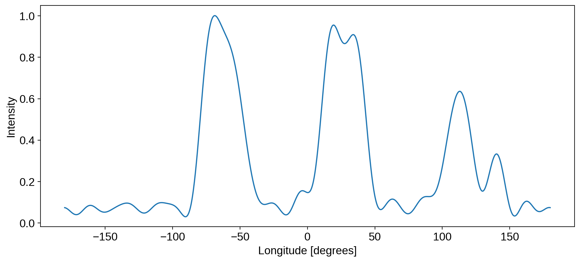
We can easily identify the Pacific (dark), South American (bright), the Atlantic (dark), Africa (bright), the Indian Ocean (dark), and Australia (bright).
Computing the flux: phase curves
The starry code is all about modeling light curves, so let’s generate some. We’ll talk about phase curves first, in which the observed flux is simply the integral over the entire disk when the object is viewed at a particular phase. Flux computations are done via the flux() method, and the phase is specified via the theta keyword:
[27]:
theta = np.linspace(0, 360, 1000)
plt.figure(figsize=(12, 5))
plt.plot(theta, map.flux(theta=theta))
plt.xlabel("Rotational phase [degrees]", fontsize=20)
plt.ylabel("Flux [normalized]", fontsize=20);
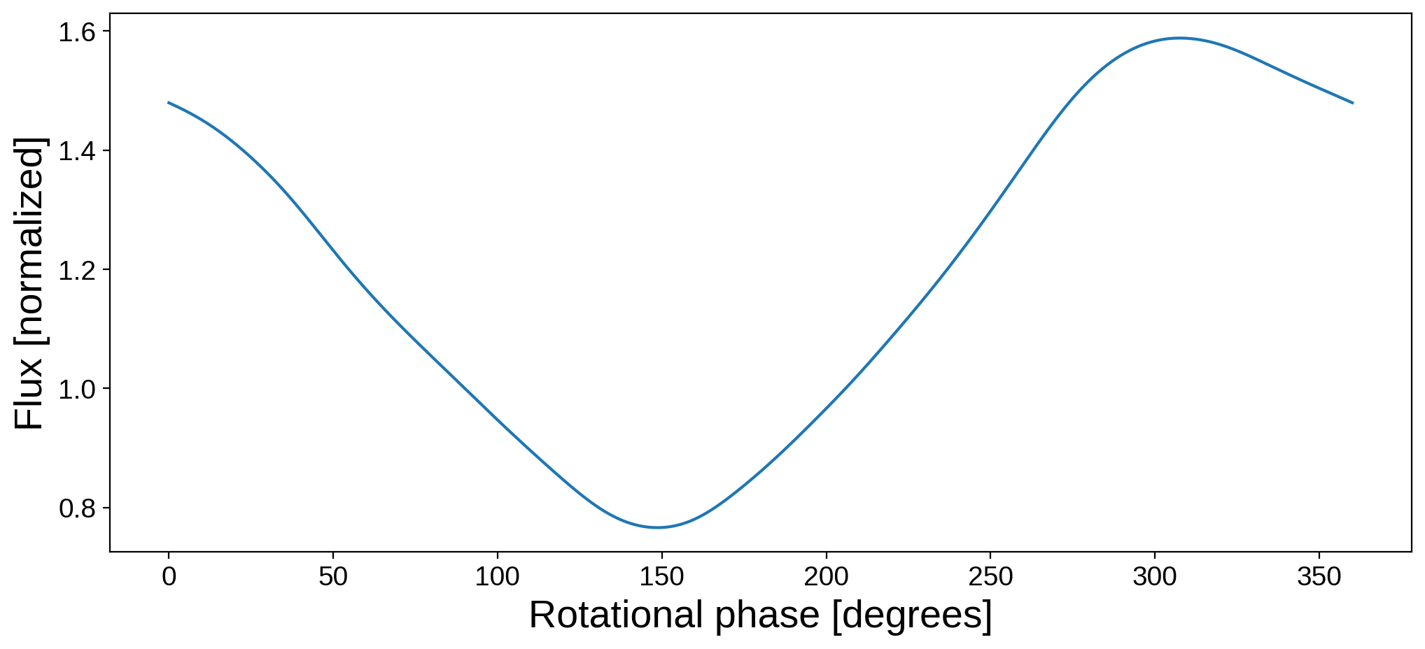
Note that this phase curve corresponds to rotation about the axis of the map, which is inclined and rotated as we specified above. We are therefore computing the disk-integrated intensity at each frame of the following animation:
[28]:
map.show(theta=np.linspace(0, 360, 50))
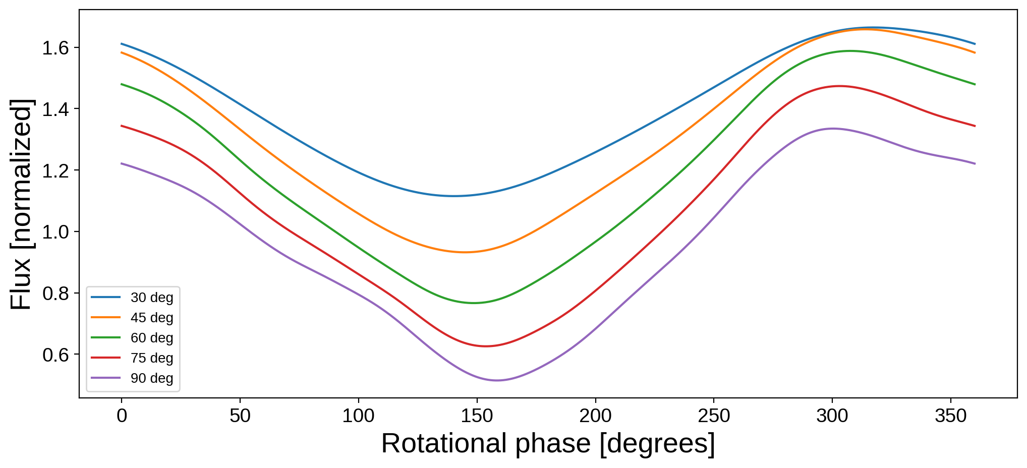
Changing the orientation of the map will change the phase curve we compute. Here’s the phase curve of the Earth at different values of the inclination:
[29]:
plt.figure(figsize=(12, 5))
for inc in [30, 45, 60, 75, 90]:
    map.inc = inc
    plt.plot(theta, map.flux(theta=theta), label="%2d deg" % inc)
plt.legend(fontsize=10)
plt.xlabel("Rotational phase [degrees]", fontsize=20)
plt.ylabel("Flux [normalized]", fontsize=20);
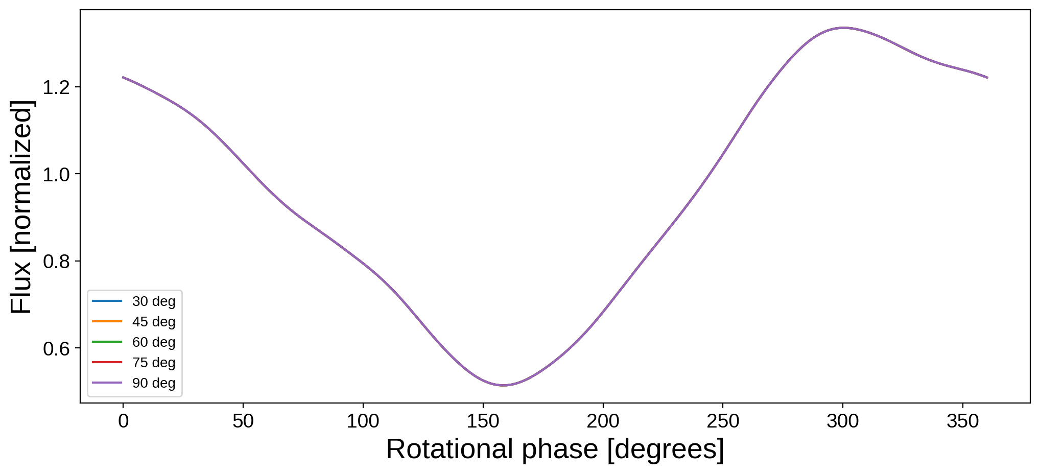
Trivially, changing the obliquity does not affect the phase curve:
[30]:
plt.figure(figsize=(12, 5))
for obl in [30, 45, 60, 75, 90]:
    map.obl = obl
    plt.plot(theta, map.flux(theta=theta), label="%2d deg" % obl)
plt.legend(fontsize=10)
plt.xlabel("Rotational phase [degrees]", fontsize=20)
plt.ylabel("Flux [normalized]", fontsize=20);
Computing the flux: transits and occultations
The spherical harmonic formalism in starry makes it easy to compute occultation light curves, since all the integrals are analytic! If we peek at the docstring for the flux method, we’ll see that it takes four parameters in addition to the rotational phase theta:
[31]:
print(map.flux.__doc__)
        Compute and return the light curve.

        Args:
            xo (scalar or vector, optional): x coordinate of the occultor
                relative to this body in units of this body's radius.
            yo (scalar or vector, optional): y coordinate of the occultor
                relative to this body in units of this body's radius.
            zo (scalar or vector, optional): z coordinate of the occultor
                relative to this body in units of this body's radius.
            ro (scalar, optional): Radius of the occultor in units of
                this body's radius.
            theta (scalar or vector, optional): Angular phase of the body
                in units of :py:attr:`angle_unit`.
            integrated (bool, optional): If True, dots the flux with the
                amplitude. Default False, in which case this returns a
                2d array (wavelength-dependent maps only).
We can pass in the Cartesian position of an occultor (xo, yo, zo) and its radius, all in units of the occulted body’s radius. Let’s use this to construct a light curve of the moon occulting the Earth:
[32]:
# Set the occultor trajectory
npts = 1000
time = np.linspace(0, 1, npts)
xo = np.linspace(-2.0, 2.0, npts)
yo = np.linspace(-0.3, 0.3, npts)
zo = 1.0
ro = 0.272
# Load the map of the Earth
map = starry.Map(ydeg=20)
map.load("earth", sigma=0.08)
# Compute and plot the light curve
plt.figure(figsize=(12, 5))
flux_moon = map.flux(xo=xo, yo=yo, ro=ro, zo=zo)
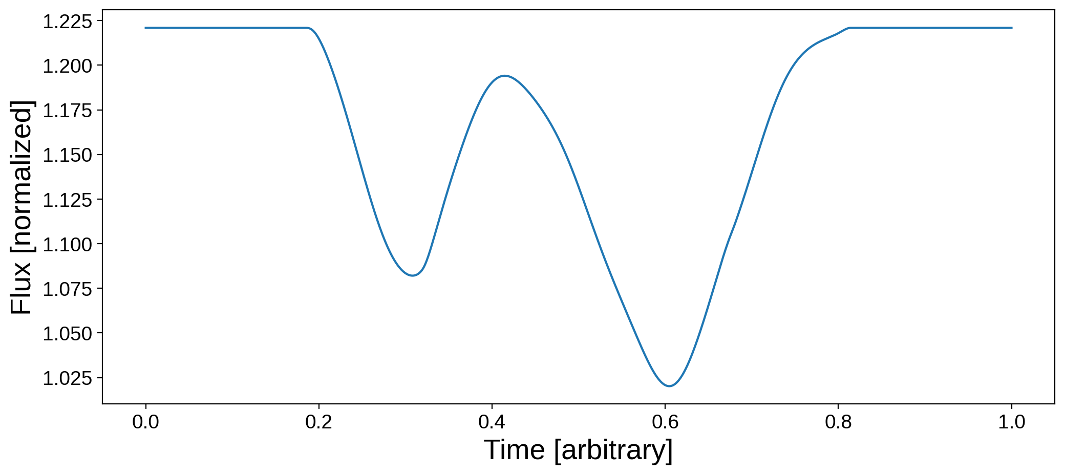
plt.plot(time, flux_moon)
plt.xlabel("Time [arbitrary]", fontsize=20)
plt.ylabel("Flux [normalized]", fontsize=20);
For reference, here is the trajectory of the occultor:
[33]:
fig, ax = plt.subplots(1, figsize=(5, 5))
ax.set_xlim(-2, 2)
ax.set_ylim(-2, 2)
ax.axis("off")
ax.imshow(map.render(), origin="lower", cmap="plasma", extent=(-1, 1, -1, 1))
for n in list(range(0, npts, npts // 10)) + [npts - 1]:
    circ = plt.Circle(
        (xo[n], yo[n]), radius=ro, color="k", fill=True, clip_on=False, alpha=0.5
    )
    ax.add_patch(circ)
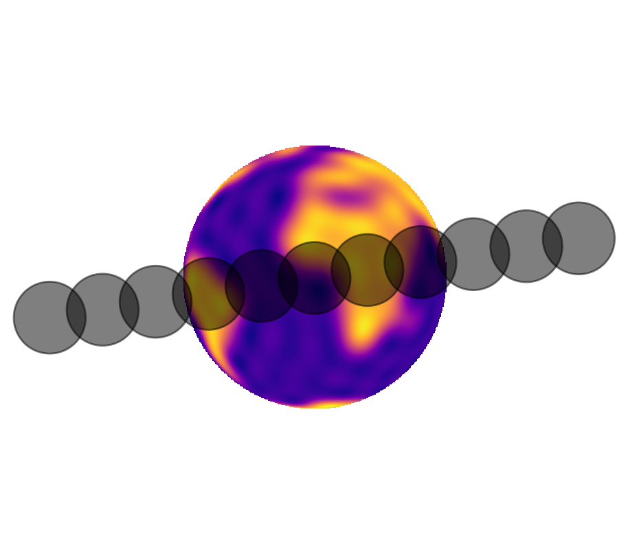
The two dips are due to occultations of South America and Africa; the bump in the middle of the transit is the moon crossing over the dark waters of the Atlantic!
Computing the flux: limb-darkening
There’s a separate tutorial on limb darkening, so we’ll just mention it briefly here. It’s super easy to add limb darkening to maps in starry. The most common reason for doing this is for modeling transits of planets across stars. To enable limb darkening, set the udeg parameter to the degree of the limb darkening model when instantiating a map. For quadratic limb darkening, we would do the following:
[34]:
map = starry.Map(udeg=2)
Setting the limb darkening coefficients is similar to setting the spherical harmonic coefficients, except only a single index is used. For instance:
[35]:
map[1] = 0.5
map[2] = 0.25
This sets the linear limb darkening coefficient to be \(u_1 = 0.5\) and the quadratic limb darkening coefficient to be \(u_2 = 0.25\) (the zeroth order coefficient, map[0], is determined by the normalization and cannot be set). Let’s look at the map:
[36]:
map.show()
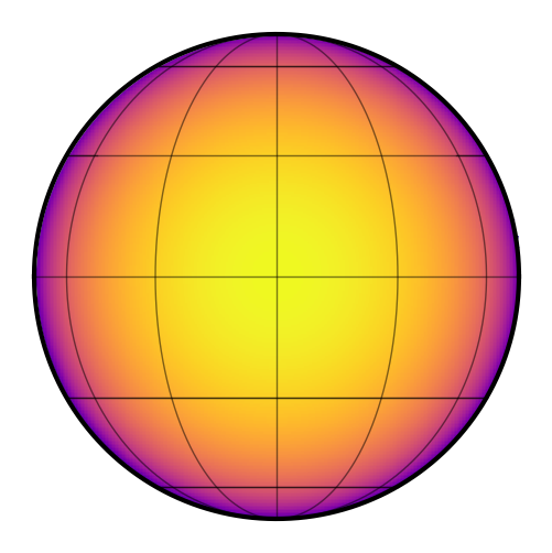
The effect of limb darkening is clear! Let’s plot a transit across this object:
[37]:
# Set the occultor trajectory
npts = 1000
time = np.linspace(0, 1, npts)
xo = np.linspace(-2.0, 2.0, npts)
yo = np.linspace(-0.3, 0.3, npts)
zo = 1.0
ro = 0.272

# Compute and plot the light curve
plt.figure(figsize=(12, 5))
plt.plot(time, map.flux(xo=xo, yo=yo, ro=ro, zo=zo))
plt.xlabel("Time [arbitrary]", fontsize=20)
plt.ylabel("Flux [normalized]", fontsize=20);
That’s it! Note that starry also allows the user to mix spherical harmonics and limb darkening, so you may set both the ydeg and udeg parameters simultaneously. Let’s look at a limb-darkened version of the Earth map, just for fun:
[38]:
map = starry.Map(ydeg=20, udeg=2)
map.load("earth", sigma=0.08)
map[1] = 0.5
map[2] = 0.25
map.show()
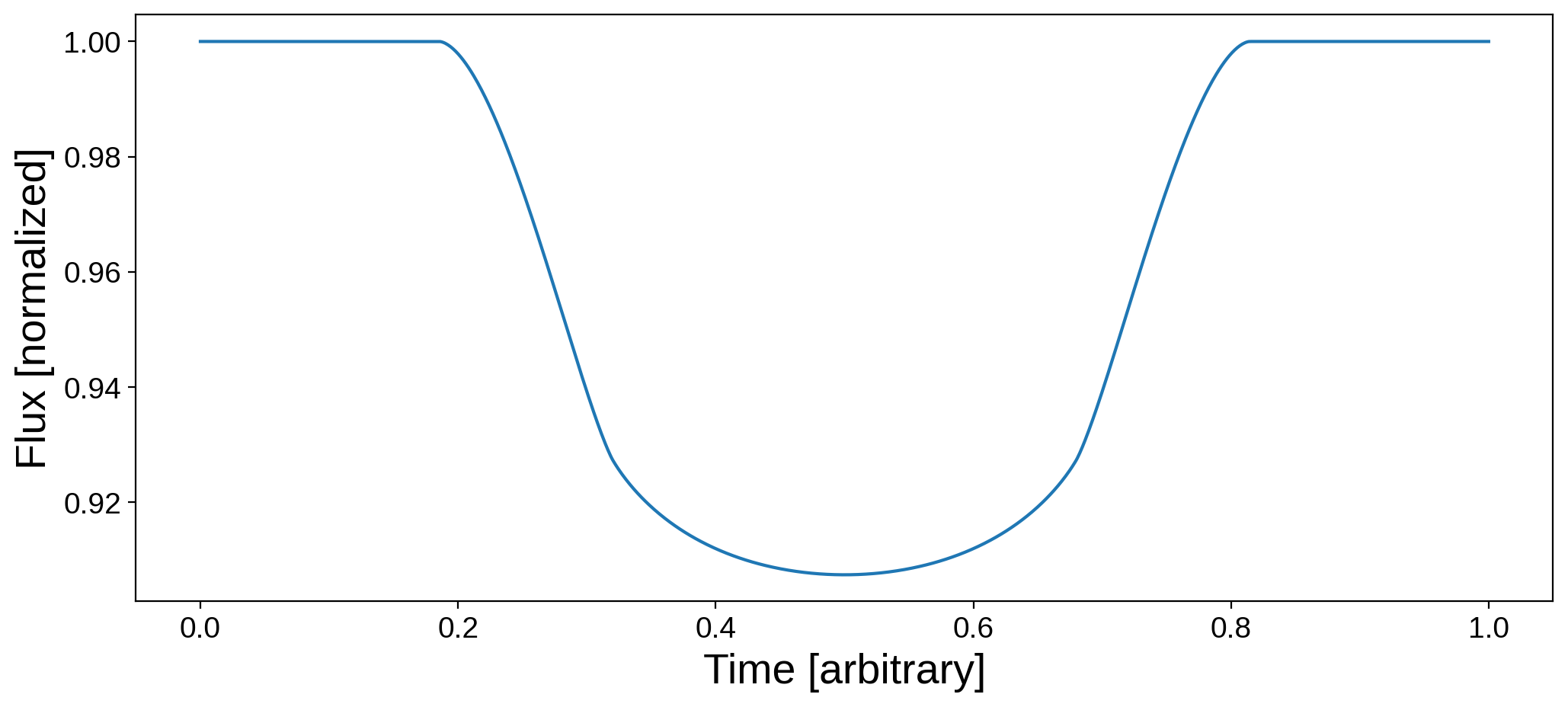
Notice how the limb is now darker! Let’s compute the transit light curve of the moon as before and compare it to the non-limb-darkened version:
[39]:
# Set the occultor trajectory
npts = 1000
time = np.linspace(0, 1, npts)
xo = np.linspace(-2.0, 2.0, npts)
yo = np.linspace(-0.3, 0.3, npts)
zo = 1.0
ro = 0.272

# Set the map inclination and obliquity
map.inc = 90
map.obl = 0

# Compute and plot the light curve
plt.figure(figsize=(12, 5))
plt.plot(time, flux_moon, label="Limb darkening off")
plt.plot(time, map.flux(xo=xo, yo=yo, ro=ro, zo=zo), label="Limb darkening on")
plt.xlabel("Time [arbitrary]", fontsize=20)
plt.ylabel("Flux [normalized]", fontsize=20)
plt.legend();
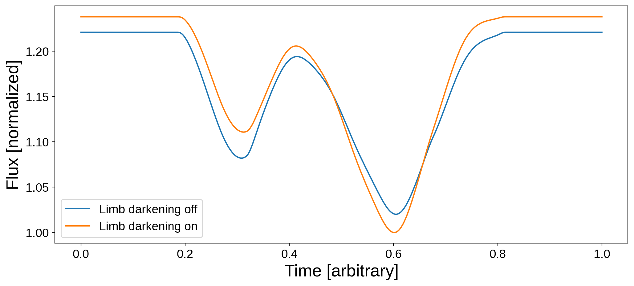
A few things are different:
The normalization changed! The limb-darkened map is slightly brighter when viewed from this orientation. In
starry, limb darkening conserves the total luminosity, so there will be other orientations at which the Earth will look dimmer;The relative depths of the two dips change, since South America and Africa receive different weightings;
The limb-darkened light curve is slightly smoother.
That’s it for this introductory tutorial. There’s a LOT more you can do with starry, including incorporating it into exoplanet to model full planetary systems, computing multi-wavelength light curves, modeling the Rossiter-McLaughlin effect, doing fast probabibilistic inference, etc.
Make sure to check out the other examples in this directory.