Note
This tutorial was generated from a Jupyter notebook that can be downloaded here.
Dimensionality Reduction
Tricks to speed up inference by projecting out of the null space!
[3]:
import numpy as np
import matplotlib.pyplot as plt
import starry
from scipy.linalg import svd
from scipy.linalg import cho_factor, cho_solve
import time
from tqdm.notebook import tqdm
[4]:
starry.config.lazy = False
starry.config.quiet = True
Generate a light curve
Let’s generate a rotational light curve to simulate a quarter of Kepler data. We’ll use a degree 10 map and give it an inclination of 60 degrees and a period of just over 30 days.
[5]:
# Instantiate a map
map = starry.Map(10, inc=60)

# The time array
t = np.arange(0, 90, 1.0 / 48.0)

# Compute the design matrix
prot = 32.234234
theta = 360.0 / prot * t
X = map.design_matrix(theta=theta)
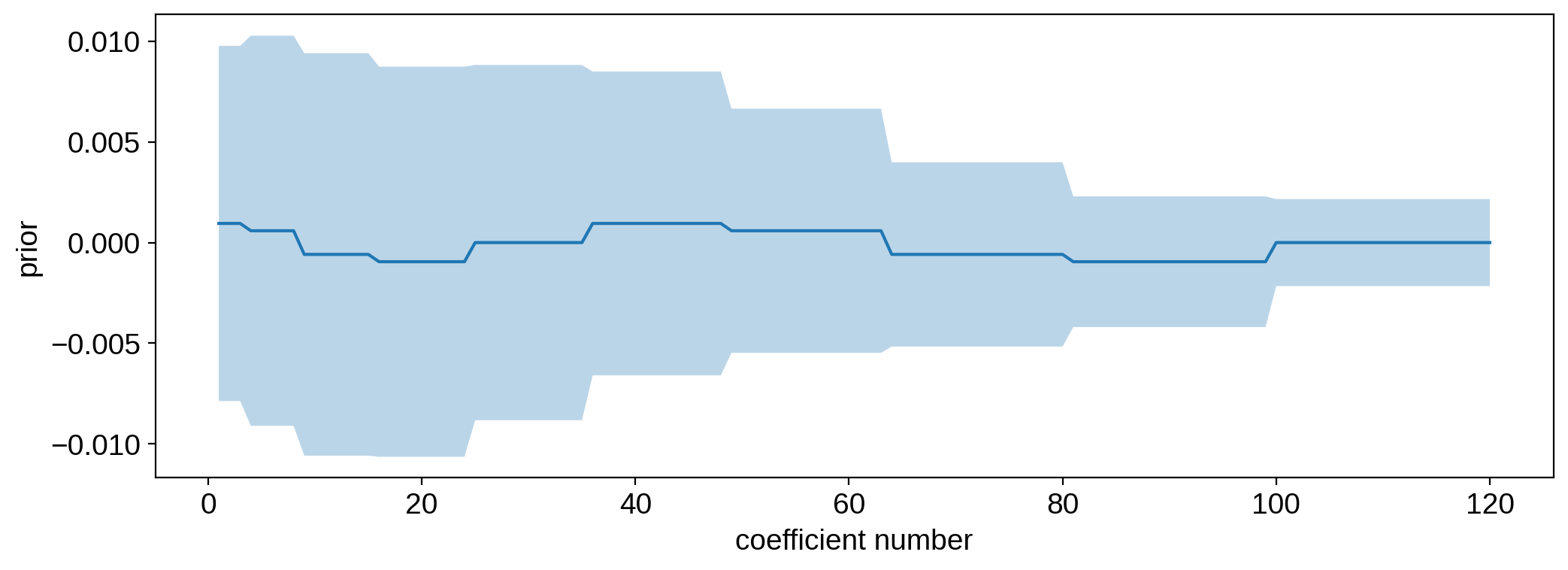
We’ll draw random coefficients from a multidimensional Gaussian with a rather arbitrary mean and covariance given by:
[6]:
# Generate random map coefficients with mean `mu` and covariance `cov`
l = np.concatenate([np.repeat(l, 2 * l + 1) for l in range(map.ydeg + 1)])
mu = 1e-3 * np.sin(2 * np.pi / 5 * l)
mu[0] = 1.0
cov = np.diag(1e-4 * np.exp(-(((l - 3) / 4) ** 2)))
cov[0, 0] = 1e-15
[7]:
plt.plot(np.arange(1, map.Ny), mu[1:])
plt.fill_between(
    np.arange(1, map.Ny),
    mu[1:] - np.sqrt(np.diag(cov)[1:]),
    mu[1:] + np.sqrt(np.diag(cov)[1:]),
    alpha=0.3,
)
plt.xlabel("coefficient number")
plt.ylabel("prior");
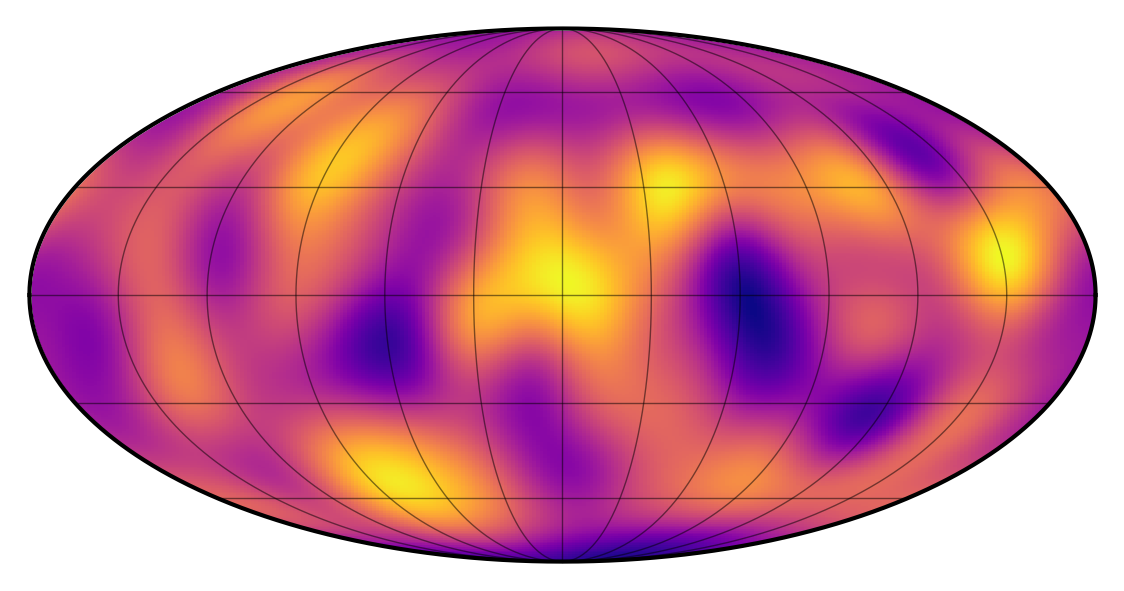
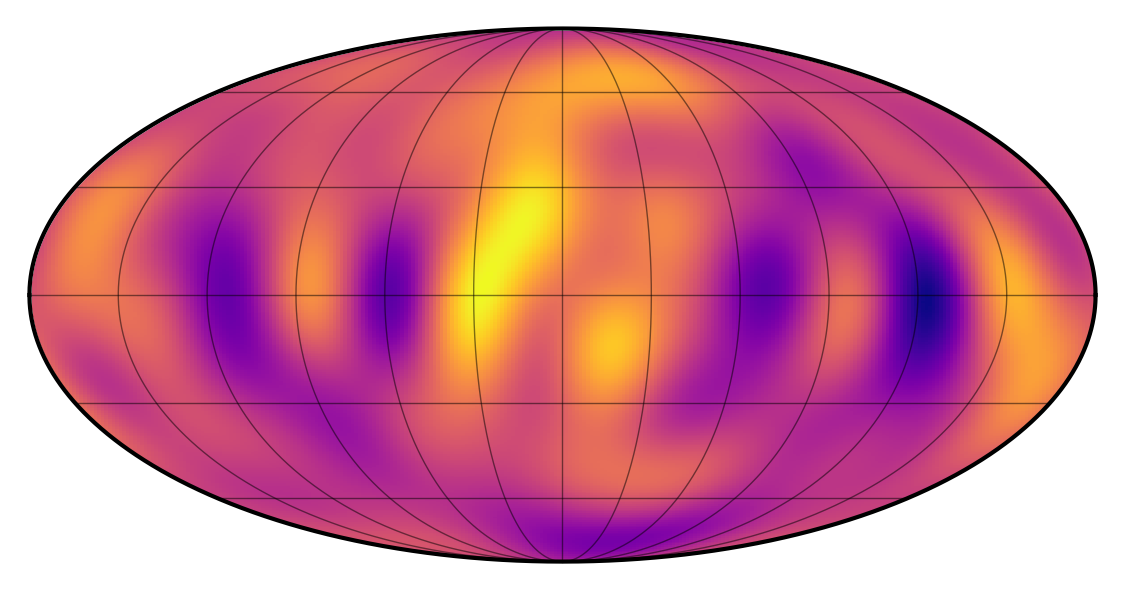
Let’s draw one sample and use that as our true map:
[8]:
np.random.seed(0)
y = np.random.multivariate_normal(mu, cov)
map[:, :] = y
map.show(projection="moll")
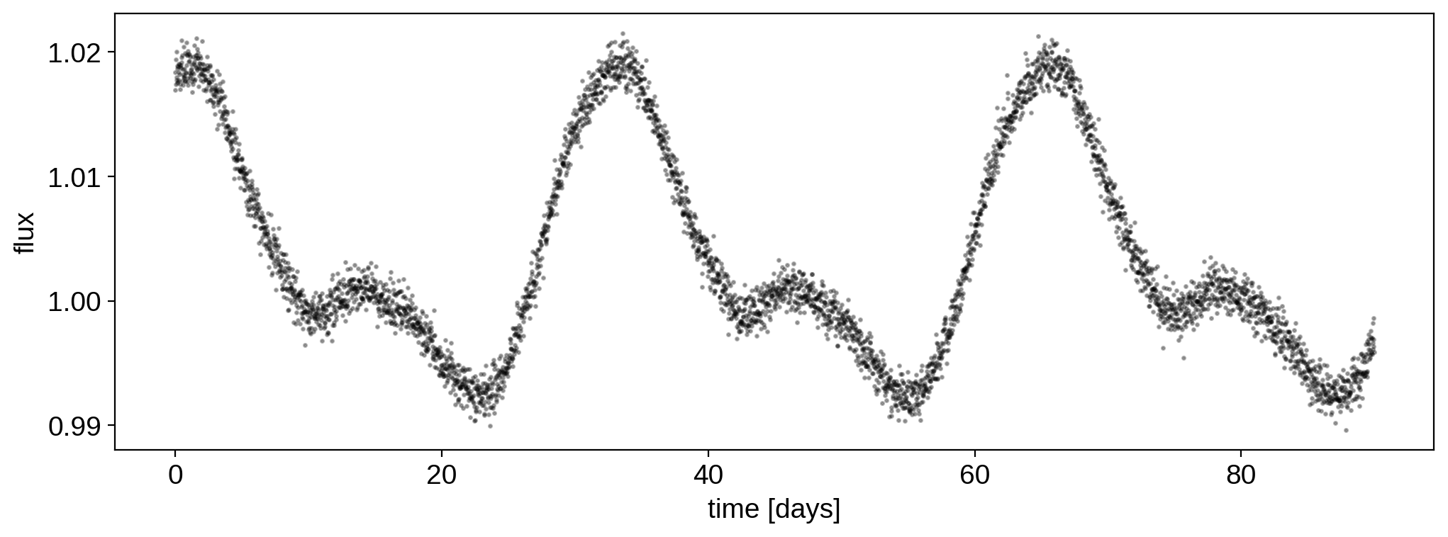
We computed the design matrix above, so getting the light curve is easy:
[9]:
# Generate the light curve with photometric error `ferr`
ferr = 1e-3
flux = X.dot(y) + ferr * np.random.randn(len(t))
[10]:
plt.plot(t, flux, "k.", alpha=0.3, ms=3)
plt.xlabel("time [days]")
plt.ylabel("flux");
Linear solve
If we know the design matrix (i.e., we know the rotational period and the inclination), inferring the surface map is simple, since the problem is linear. For simplicity, let’s assume we actually know the true mean mu and variance cov of the process.
[11]:
# Solve the linear problem
# `yhat` is the posterior mean, and
# `cho_ycov` is the Cholesky decomposition of the posterior covariance
yhat, cho_ycov = starry.linalg.solve(X, flux, C=ferr ** 2, mu=mu, L=cov)
We can look at the map corresponding to the posterior mean:
[12]:
map[:, :] = yhat
map.show(projection="moll")

It doesn’t really look like the true map, but you can convince yourself that some of the spots are actually in the correct place. This is particularly true right near the equator. The problem with the southern latitudes is that they are never in view (since the star is inclined toward us); conversely, the northern latitudes are always in view, so their features don’t really affect the flux as the star rotates.
Another way to think about this is that the problem of inferring a map from a rotational light curve is extremely ill-conditioned: it has a very large null space, meaning most of the modes on the surface do not affect the flux whatsoever.
To verify this, check out the rank of the design matrix:
[13]:
rank = np.linalg.matrix_rank(X)
rank
[13]:
21
It’s only 21, even though the dimensions of the matrix are
[14]:
X.shape
[14]:
(4320, 121)
The number to compare to here is the number of columns: 121. That’s the number of spherical harmonic coefficients we’re trying to infer. However, the matrix rank tells us that the flux operator X only uses information from (effectively) 21 of those coefficients when producing a light curve. This isn’t an issue with starry: this is a fundamental limitation of rotational light curves, since they simply don’t encode that much information about the surface.
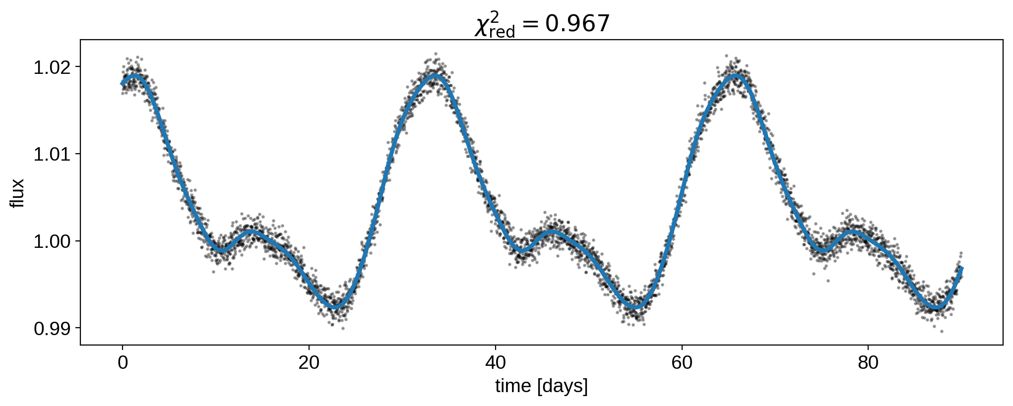
Anyways, even though the inferred map looks quite different from the true map, we can verify that the light curve we get from the inferred map is indistinguishable from the data:
[15]:
plt.plot(t, flux, "k.", alpha=0.3, ms=3)
plt.plot(t, map.flux(theta=theta), lw=3)
plt.xlabel("time [days]")
plt.ylabel("flux")
plt.title(
    r"$\chi^2_\mathrm{red} = %.3f$"
    % (np.sum((flux - map.flux(theta=theta)) ** 2 / ferr ** 2) / (len(t) - rank))
);

This is evidence, again, of the crazy degeneracies at play.
Taking advantage of the null space
The null space is a huge hassle, since it limits how much we can learn about a surface from a light curve. But it can also be advantageous, in one sense at least: we can exploit it to greatly speed up our computations. In our linear solve step above, we’re solving for 121 coefficients (which amounts to inverting a 121x121 matrix), even though we can only hope to constrain 21 of them. We certainly do obtain values for all of them, but most of the information in our posterior is
coming from our prior.
Here’s the trick. With a bit of linear algebra, we can transform our problem into a smaller space of dimension 21 that has no null space. We can solve the problem in that space (i.e., invert a 21x21 matrix), then project out of it and fill in the remaining coefficients with our prior.
I’ll explain more below, but all of this is really similar to what Emily Rauscher et al. did in their 2018 paper on eclipse mapping, so check that out if you’re interested.
SVD to the rescue
The basic idea behind our trick is to use singular value decomposition (SVD; read about it here). This is closely related to principal component analysis (PCA). We’re going to use SVD to identify the 21 coefficients (or linear combinations of coefficients) that can be constrained from the data and trim the remaining ones (i.e., the ones in the null space).
It’s probably easiest if we just dive straight in. We’ll use the svd function from scipy.linalg:
[16]:
U, s, VT = svd(X)
S = np.pad(np.diag(s), ((0, U.shape[1] - s.shape[0]), (0, 0)))
We now have three matrices U, S, and V^T. Note that S is a diagonal matrix (svd returns it as an array, so we need to massage it a bit to get the dimensions correct). The thing to note here is that the dot product of these three matrices is equal to (within numerical precision) to the design matrix X:
[17]:
np.allclose(U @ S @ VT, X)
[17]:
True
Now let’s look at the diagonal entries in the matrix S:
[18]:
plt.plot(np.diag(S))
plt.axvline(rank, color="C1")
plt.yscale("log");
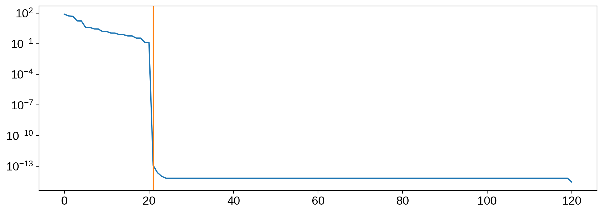
These are called the singular values of X; they are the contribution from each basis vector in U. Note the extremely steep drop after the 21st singular value: that’s the null space! All columns in U beyond 21 contribute effectively nothing to X. The same is true for all rows in VT beyond 21. We can verify this by removing them:
[19]:
U = U[:, :rank]
S = S[:rank, :rank]
VT = VT[:rank, :]
[20]:
np.allclose(U @ S @ VT, X)
[20]:
True
As promised, we can just get rid of them and still reconstruct X exactly. Let’s now inspect the U matrix:
[21]:
plt.imshow(U, aspect="auto");
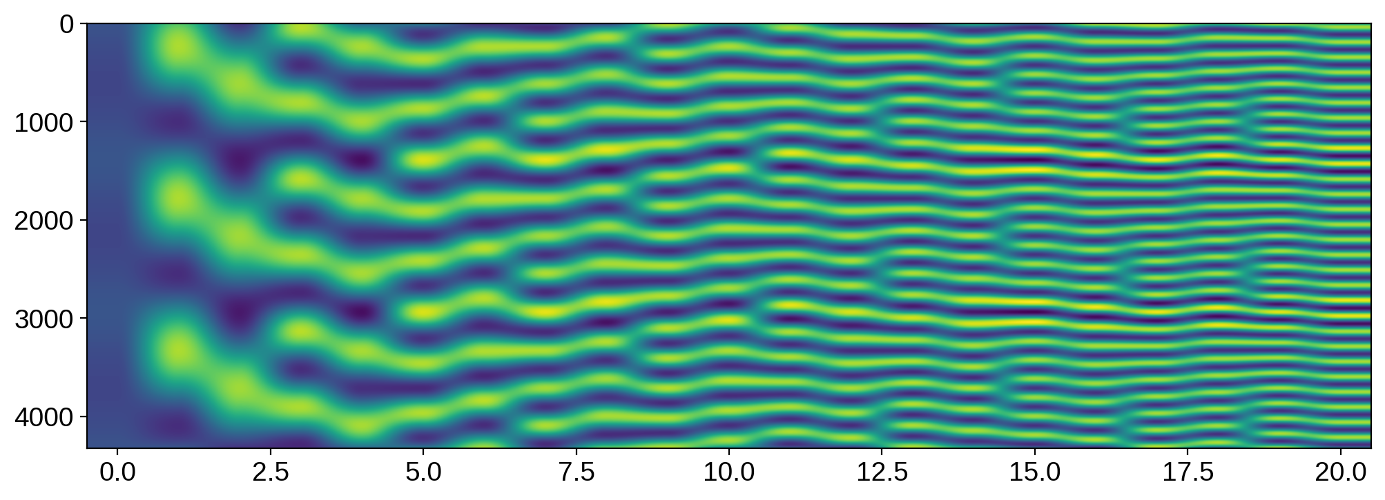
Its columns are the principal components of X. Note, importantly, the perfect periodicity among them; in fact, these are exactly sines and cosines!
Here’s the punchline, which is perhaps obvious in hindsight: the only signals that a rotating, spherical body can contribute to the disk-integrated flux are a sine and a cosine corresponding to each spatial frequency. Therefore, a map of spherical harmonic degree lmax will contribute lmax sines and lmax cosines (plus one DC offset term), for a total of 2 * lmax + 1 terms. Our map has degree 10, so it now makes sense why we can only constrain 21 terms!
Now let’s look at the VT matrix:
[22]:
plt.imshow(VT, aspect="auto");
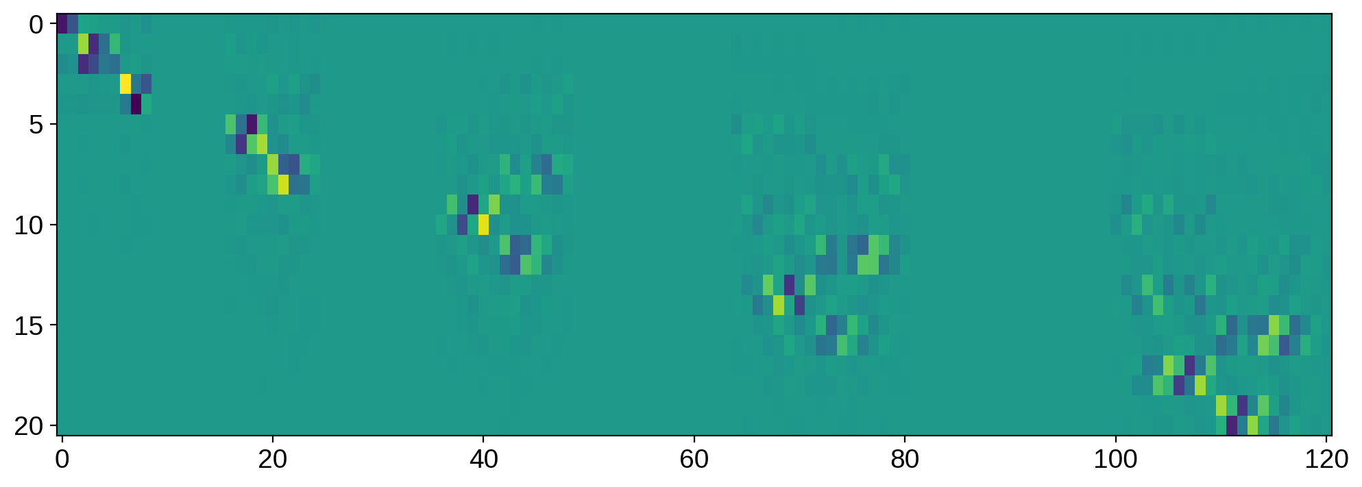
The rows of this matrix tell us which linear combinations of the spherical harmonic vector give us the sine and cosine terms in U. There are lots of things to note here, but perhaps the most obvious one is that there are columns that are zero everywhere: they correspond to coefficients that are in the null space. Most of the other terms in the null space correspond to linear combinations of coefficients (which are harder to visualize).
Linear solve with no null space
Now that we’ve done SVD, our job is basically done. The magic is all in the VT matrix and its transpose:
[23]:
V = VT.T
The VT matrix is actually the projection operator that takes us from spherical harmonic space to the magical space in which we’ll do our inference. Its transpose will then take us back to spherical harmonic space.
The first thing we’ll do is project our design matrix into the compact space we’ll do inference in.
[24]:
X_V = X.dot(V)
Note that our design matrix now has shape
[25]:
X_V.shape
[25]:
(4320, 21)
i.e., 21 columns, meaning we’ll only need to invert a 21x21 matrix during the solve step. The solve is the same as before:
[26]:
# Solve the linear problem
yhat_V, cho_ycov_V = starry.linalg.solve(
    X_V, flux, C=ferr ** 2, mu=0, L=1e12, N=X_V.shape[1]
)
Our posterior mean and covariance are in the compact space. We need to project them back to spherical harmonic space and fill in the missing data from our prior. Here’s the linear algebra to do just that:
[27]:
# Transform the mean back to Ylm space
yhat2, cho_ycov2 = starry.linalg.solve(V.T, yhat_V, cho_C=cho_ycov_V, mu=mu, L=cov)
We can verify our posterior map is very similar to the one we obtained above:
[28]:
map[:, :] = yhat2
map.show(projection="moll")
And check that we get the correct flux model (with the exact same likelihood):
[29]:
plt.plot(t, flux, "k.", alpha=0.3, ms=3)
plt.plot(t, map.flux(theta=theta), lw=3)
plt.xlabel("time [days]")
plt.ylabel("flux")
plt.title(
    r"$\chi^2_\mathrm{red} = %.3f$"
    % (np.sum((flux - map.flux(theta=theta)) ** 2 / ferr ** 2) / (len(t) - rank))
);
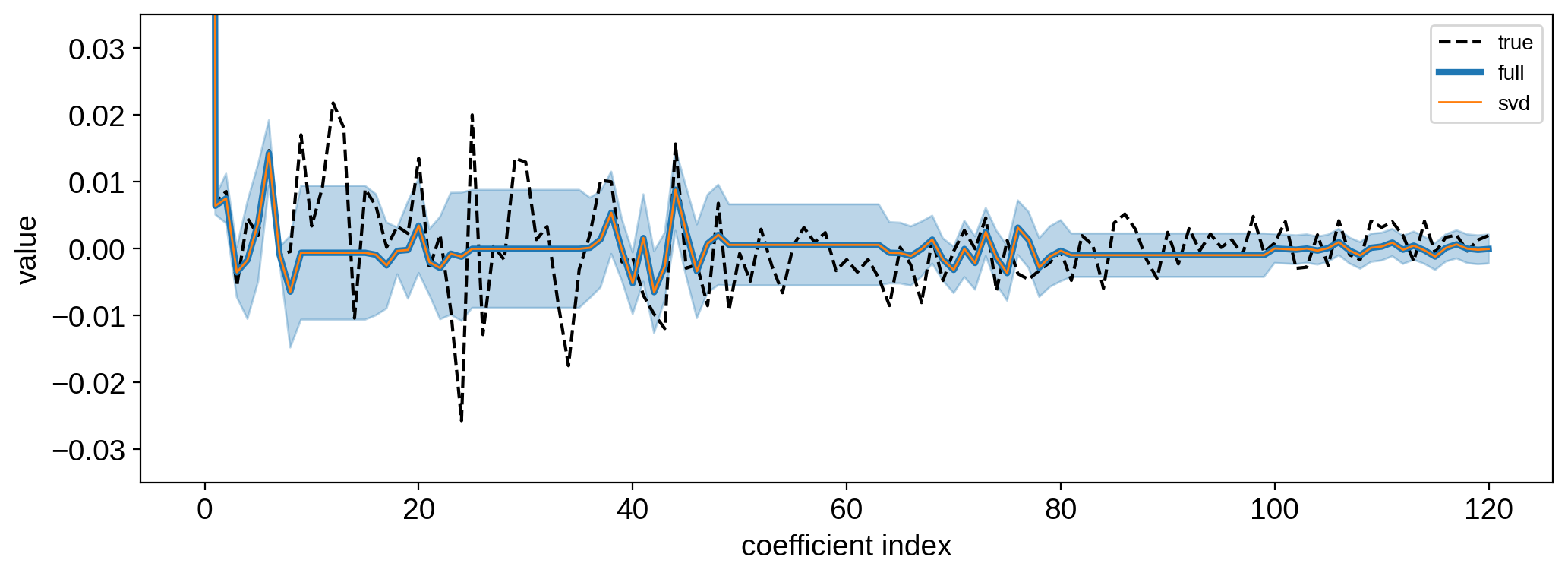
We can further compare our posterior mean coefficients:
[30]:
plt.plot(y, "k--", label="true")
plt.plot(yhat, lw=3, label="full")
plt.plot(yhat2, lw=1, label="svd")
std = np.sqrt(np.diag(cho_ycov.dot(cho_ycov.T)))
plt.fill_between(np.arange(len(yhat)), yhat - std, yhat + std, color="C0", alpha=0.3)
plt.legend(fontsize=10)
plt.xlabel("coefficient index")
plt.ylabel("value")
plt.ylim(-0.035, 0.035);
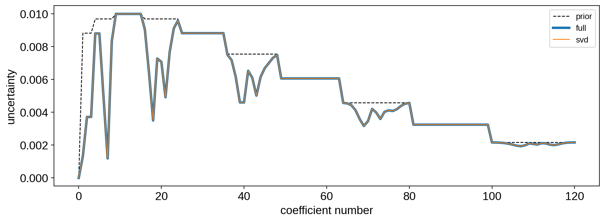
As well as the posterior covariance:
[31]:
# Get the posterior covariance
ycov = np.tril(cho_ycov).dot(np.tril(cho_ycov).T) + 1e-15
ycov2 = np.tril(cho_ycov2).dot(np.tril(cho_ycov2).T) + 1e-15

fig, ax = plt.subplots(1, 2, figsize=(8, 4))
ax[0].imshow(np.log10(np.abs(ycov)), vmin=-15, vmax=0)
ax[1].imshow(np.log10(np.abs(ycov2)), vmin=-15, vmax=0)

plt.figure()
plt.plot(np.sqrt(np.diag(cov)), "k--", lw=1, label="prior")
plt.plot(np.sqrt(np.diag(ycov)), lw=3, label="full")
plt.plot(np.sqrt(np.diag(ycov2)), lw=1, label="svd")
plt.legend(fontsize=10)
plt.xlabel("coefficient number")
plt.ylabel("uncertainty");

If you were paying close attention, there are small differences in the results we get using SVD. Even though our fit to the data is just as good, the maps don’t look quite the same. There are some subtle numerical issues at play here, but keep in mind that the disagreement is small and restricted entirely to the null space, so it’s not really an issue.
An even better way of doing this
We showed how to solve the light curve problem in a more compact space – saving us precious flops. However, we introduced several extra matrix multiplications, as well as the (quite costly) SVD step. Fortunately, we can actually skip SVD entirely. That’s because we know that the representation of the compact basis in flux space is just sines and cosines. So, instead of doing SVD (which is nonlinear and slow), we can cast the problem as a (small) matrix inversion instead.
First, construct a tiny design matrix that spans one rotation. We’re going to do the equivalent of SVD on this small matrix to get our change-of-basis matrix V as before.
[32]:
K = rank + 1
theta = np.linspace(0, 2 * np.pi, K, endpoint=False)
A = map.design_matrix(theta=theta * 180 / np.pi)
Note that the number of rows in this matrix is one more than its rank (so that it’s well-conditioned).
As we mentioned above, we know that the U matrix in the SVD problem is just sines and cosines, so we can explicitly construct it:
[33]:
theta = theta.reshape(-1, 1)
U = np.hstack(
    [np.ones_like(theta)]
    + [
        np.hstack([np.cos(n * theta), np.sin(n * theta)])
        for n in range(1, map.ydeg + 1)
    ]
)
We can now solve the equation U @ VT = A for VT:
[34]:
cho_U = cho_factor(U.T.dot(U))
Z = cho_solve(cho_U, U.T)
VT = Z @ A
Finally, since we didn’t account for the S matrix above, we need to normalize VT so that its dot product with its transpose is the identity (which ensures the basis is orthonormal):
[35]:
VT /= np.sqrt(np.diag(VT.dot(VT.T))).reshape(-1, 1)
V = VT.T
Now, we can speed up the inference step by simplifying a bit of the linear algebra. Note that we have two solve steps: one to do inference in the compact space, and one to project back to the spherical harmonic space. We can combine the two steps into the following:
[36]:
# Solve the linear problem
X_V = X.dot(V)
yhat_V, cho_ycov_V = starry.linalg.solve(
    X_V, flux, C=ferr ** 2, mu=0, L=1e12, N=X_V.shape[1]
)
yhat3, cho_ycov3 = starry.linalg.solve(V.T, yhat_V, cho_C=cho_ycov_V, mu=mu, L=cov)
[37]:
cho_cov = cho_factor(cov, True)
inv_cov = cho_solve(cho_cov, np.eye(cov.shape[0]))

XV = X @ V
D = (V / ferr ** 2) @ XV.T

Cinv = (D @ XV) @ V.T + inv_cov
C = cho_solve(cho_factor(Cinv, True), np.eye(cov.shape[0]))

yhat3 = C @ (D @ flux + cho_solve(cho_cov, mu))
cho_ycov3, _ = cho_factor(C, True)
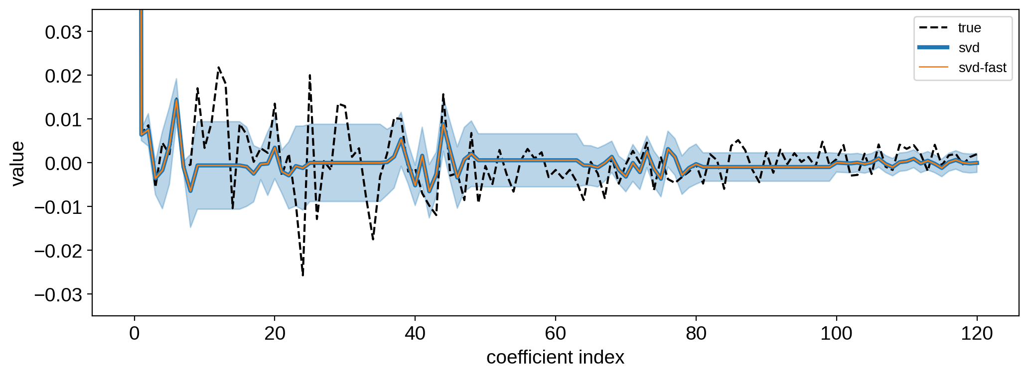
We can verify that we get the exact same result as doing SVD:
[38]:
plt.plot(y, "k--", label="true")
plt.plot(yhat2, lw=3, label="svd")
plt.plot(yhat3, lw=1, label="svd-fast")
std = np.sqrt(np.diag(cho_ycov.dot(cho_ycov.T)))
plt.fill_between(np.arange(len(yhat)), yhat - std, yhat + std, color="C0", alpha=0.3)
plt.legend(fontsize=10)
plt.xlabel("coefficient index")
plt.ylabel("value")
plt.ylim(-0.035, 0.035);
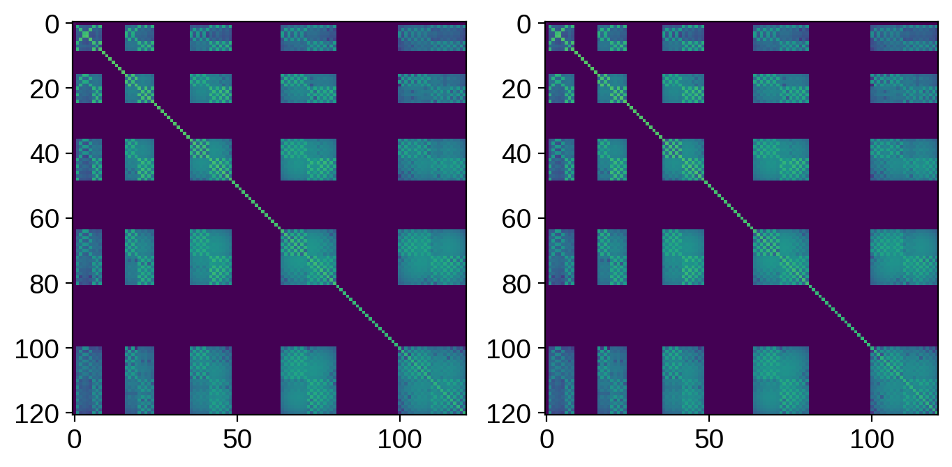
[39]:
# Get the posterior covariance
ycov = np.tril(cho_ycov2).dot(np.tril(cho_ycov2).T) + 1e-15
ycov3 = np.tril(cho_ycov3).dot(np.tril(cho_ycov3).T) + 1e-15
fig, ax = plt.subplots(1, 2, figsize=(8, 4))
ax[0].imshow(np.log10(np.abs(ycov2)), vmin=-15, vmax=0)
ax[1].imshow(np.log10(np.abs(ycov3)), vmin=-15, vmax=0)
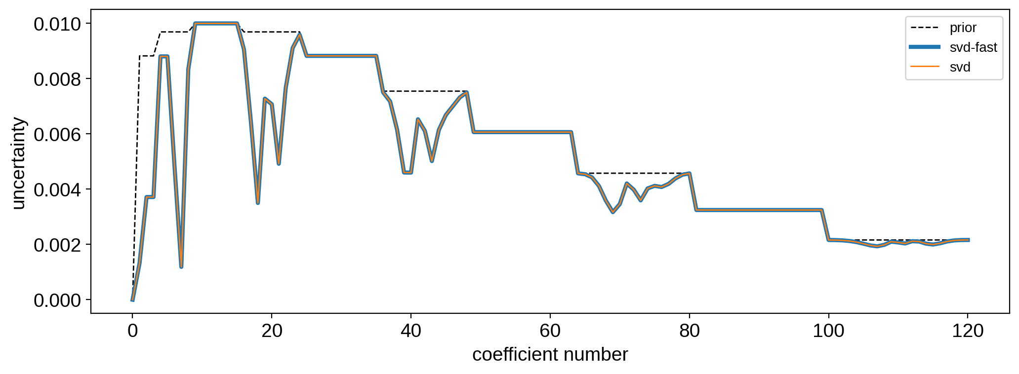
plt.figure()
plt.plot(np.sqrt(np.diag(cov)), "k--", lw=1, label="prior")
plt.plot(np.sqrt(np.diag(ycov2)), lw=3, label="svd-fast")
plt.plot(np.sqrt(np.diag(ycov3)), lw=1, label="svd")
plt.legend(fontsize=10)
plt.xlabel("coefficient number")
plt.ylabel("uncertainty");
Speed comparison
Let’s now compare the speed of these two methods. First, let’s define a class that will help us do the timing.
[40]:
class TimingTests(object):
    def __init__(self, ydeg, npts, nest=10):
        self.ydeg = ydeg
        self.npts = npts
        self.nest = nest
        self.map = starry.Map(ydeg, inc=60)
        self.t = np.linspace(0, 1, npts)

        # random data & random prior
        self.flux = np.random.randn(npts)
        self.ferr = 1.0
        self.cov = np.diag(np.random.randn(self.map.Ny) ** 2)
        self.invcov = np.linalg.inv(self.cov)
        self.mu = np.random.randn(self.map.Ny)

        # Design matrix
        self.X = self.map.design_matrix(theta=360.0 * self.t)

        # Pre-compute the Cholesky decomp of the U matrix
        K = 2 * self.ydeg + 1
        self.theta = np.linspace(0, 360.0, K, endpoint=False)
        theta_rad = self.theta.reshape(-1, 1) * np.pi / 180
        U = np.hstack(
            [np.ones_like(theta_rad)]
            + [
                np.hstack([np.cos(n * theta_rad), np.sin(n * theta_rad)])
                for n in range(1, self.ydeg + 1)
            ]
        )
        cho_U = cho_factor(U.T.dot(U))
        self.Z = cho_solve(cho_U, U.T)

    def time_full(self):

        start = time.time()
        for k in range(self.nest):

            self.yhat, self.cho_ycov = starry.linalg.solve(
                self.X, self.flux, C=self.ferr ** 2, mu=self.mu, L=self.cov
            )

        return (time.time() - start) / self.nest

    def time_fast(self):

        start = time.time()
        for k in range(self.nest):

            # Get the change-of-basis matrix
            A = self.map.design_matrix(theta=self.theta)
            VT = self.Z @ A
            VT /= np.sqrt(np.diag(VT.dot(VT.T))).reshape(-1, 1)
            V = VT.T

            # Cast the matrix to the compact space
            X_V = self.X.dot(V)

            # Solve the linear problem
            yhat_V, cho_ycov_V = starry.linalg.solve(
                X_V, self.flux, C=self.ferr ** 2, mu=0, L=1e10, N=X_V.shape[1]
            )

            # Transform back to Ylm space
            self.yhat, self.cho_ycov = starry.linalg.solve(
                V.T, yhat_V, cho_C=cho_ycov_V, mu=self.mu, L=self.cov
            )

        return (time.time() - start) / self.nest

    def time_fast_precomp(self):

        # Get the change-of-basis matrix
        A = self.map.design_matrix(theta=self.theta)
        VT = self.Z @ A
        VT /= np.sqrt(np.diag(VT.dot(VT.T))).reshape(-1, 1)
        V = VT.T

        # Cast the matrix to the compact space
        X_V = self.X.dot(V)

        start = time.time()
        for k in range(self.nest):

            # Solve the linear problem
            yhat_V, cho_ycov_V = starry.linalg.solve(
                X_V, self.flux, C=self.ferr ** 2, mu=0, L=1e10, N=X_V.shape[1]
            )

            # Transform back to Ylm space
            self.yhat, self.cho_ycov = starry.linalg.solve(
                V.T, yhat_V, cho_C=cho_ycov_V, mu=self.mu, L=self.cov
            )

        return (time.time() - start) / self.nest
Compare the two methods on a grid of spherical harmonic degree and number of points:
[41]:
ydeg = np.array(np.arange(1, 21), dtype=int)
npts = np.array(np.logspace(2, 4, 10), dtype=int)
ratio = np.ones((len(ydeg), len(npts)))
for i in tqdm(range(len(ydeg))):
    for j in range(len(npts)):
        T = TimingTests(ydeg[i], npts[j])
        ratio[i, j] = T.time_fast() / T.time_full()
[42]:
fig, ax = plt.subplots(1, figsize=(8, 6))
im = ax.imshow(
    np.log10(ratio),
    origin="lower",
    extent=(np.log10(npts[0]), np.log10(npts[-1]), ydeg[0], ydeg[-1]),
    vmin=-1,
    vmax=1,
    cmap="RdBu",
    aspect="auto",
)
cb = plt.colorbar(im)
cb.set_ticks([-1, -np.log10(3), 0, np.log10(3), 1])
cb.set_ticklabels(
    [
        r"$10\times\ \mathrm{faster}$",
        r"$3\times\ \mathrm{faster}$",
        r"$\mathrm{equal}$",
        r"$3\times\ \mathrm{slower}$",
        r"$10\times\ \mathrm{slower}$",
    ]
)
ax.set_xticks([2, 3, 4])
ax.set_xticklabels([r"$10^2$", r"$10^3$", r"$10^4$"])
ax.set_yticks([1, 5, 10, 15, 20])
ax.set_yticklabels([r"$1$", r"$5$", r"$10$", r"$15$", r"$20$"])
ax.set_xlabel("length of timeseries")
ax.set_ylabel("spherical harmonic degree")
ax.set_title("SVD trick speed test");
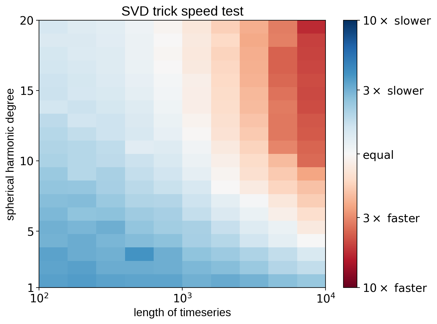
The SVD trick is slower for low spherical harmonic degree and small timeseries, but it can be much faster if ydeg is high and/or the timeseries has lots of points.
One last point: if we can pre-compute the change of basis matrix (in cases where the inclination is known or fixed), things get much better:
[43]:
ydeg = np.array(np.arange(1, 21), dtype=int)
npts = np.array(np.logspace(2, 4, 10), dtype=int)
ratio = np.ones((len(ydeg), len(npts)))
for i in tqdm(range(len(ydeg))):
    for j in range(len(npts)):
        T = TimingTests(ydeg[i], npts[j])
        ratio[i, j] = T.time_fast_precomp() / T.time_full()
[44]:
fig, ax = plt.subplots(1, figsize=(8, 6))
im = ax.imshow(
    np.log10(ratio),
    origin="lower",
    extent=(np.log10(npts[0]), np.log10(npts[-1]), ydeg[0], ydeg[-1]),
    vmin=-1,
    vmax=1,
    cmap="RdBu",
    aspect="auto",
)
cb = plt.colorbar(im)
cb.set_ticks([-1, -np.log10(3), 0, np.log10(3), 1])
cb.set_ticklabels(
    [
        r"$10\times\ \mathrm{faster}$",
        r"$3\times\ \mathrm{faster}$",
        r"$\mathrm{equal}$",
        r"$3\times\ \mathrm{slower}$",
        r"$10\times\ \mathrm{slower}$",
    ]
)
ax.set_xticks([2, 3, 4])
ax.set_xticklabels([r"$10^2$", r"$10^3$", r"$10^4$"])
ax.set_yticks([1, 5, 10, 15, 20])
ax.set_yticklabels([r"$1$", r"$5$", r"$10$", r"$15$", r"$20$"])
ax.set_xlabel("length of timeseries")
ax.set_ylabel("spherical harmonic degree")
ax.set_title("SVD trick speed test (pre-computed)");
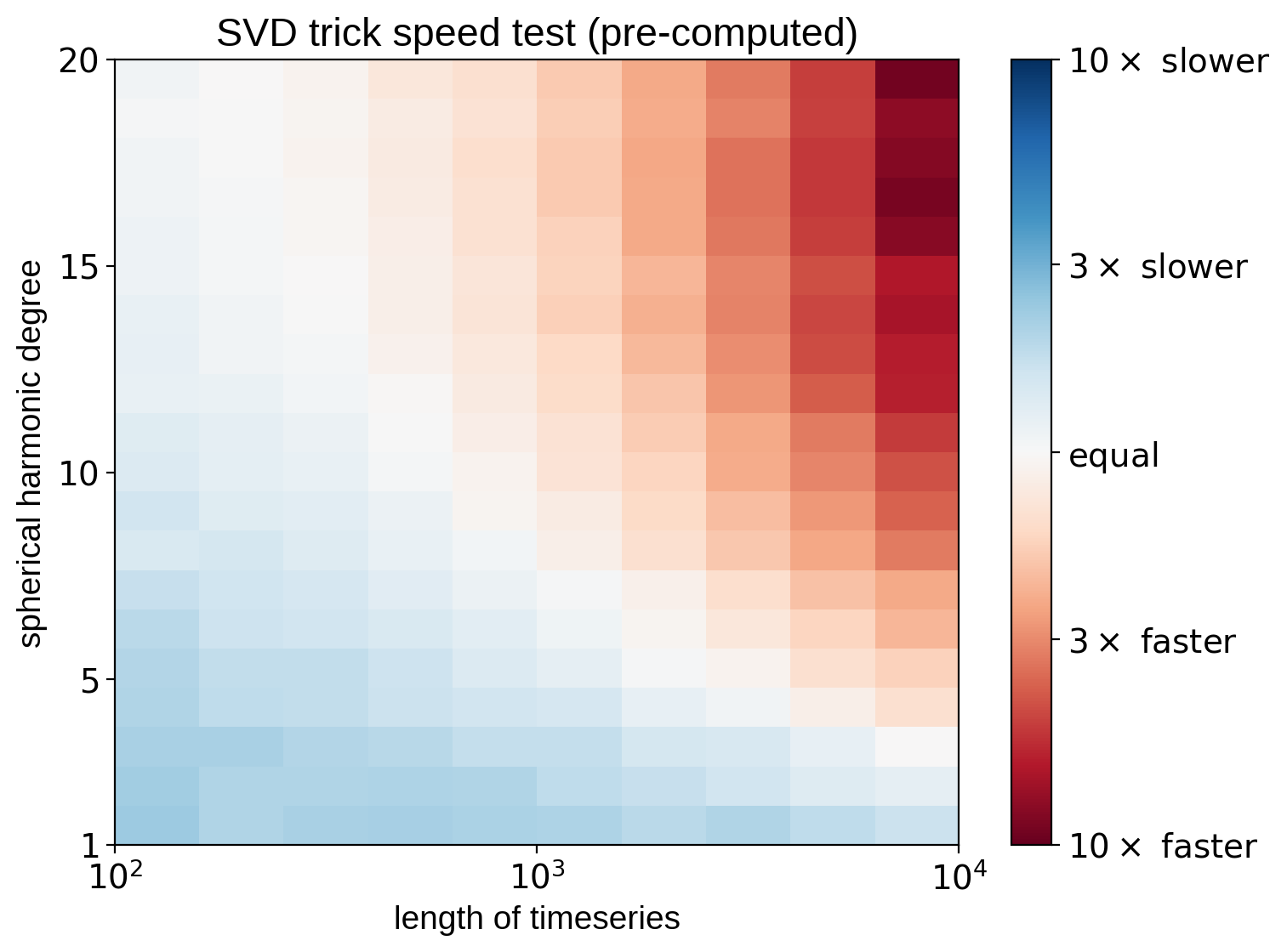
That’s it for this tutorial. Keep in mind that our trick of sidestepping the SVD computation with a fast linear solve works only in the case of rotational light curves with no limb darkening. As soon as we add limb darkening, transits, or occultations, the compact basis is no longer strictly composed of sines and cosines. We can still do dimensionality reduction, but in these cases we have to perform full SVD, which is slow. But, as we showed above, if we can pre-compute this change of basis matrix, the speed gains may still be huge.